
ML
The Binarizer transform details are provided under this section.
Binarizer
It converts the value of a numerical column to zero when the value in the column is less than or equals to the threshold value and one if the value in the column is greater than threshold value.
Check out the given illustration on how to apply Binarizer transform.
Steps to apply Binarizer transform:
Select a numeric column from the dataset.
Open the Transforms tab.
Select the Binarizer transform from the ML category of transforms.
Provide a Threshold value.
Click the Submit option.
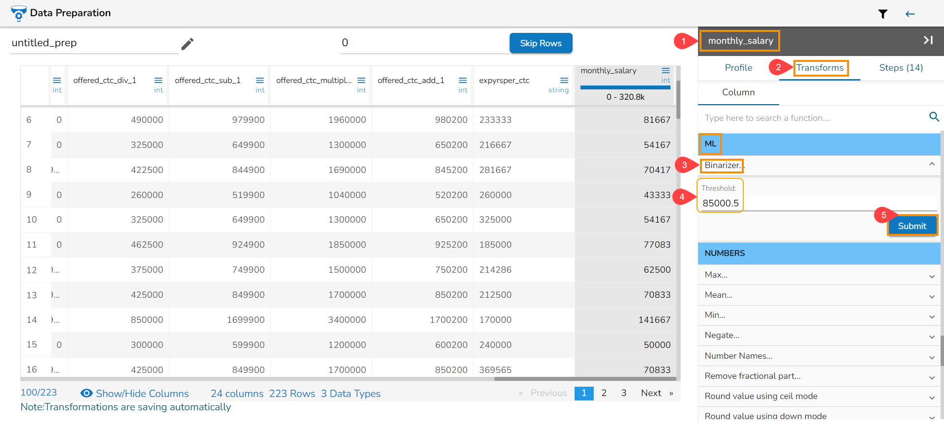
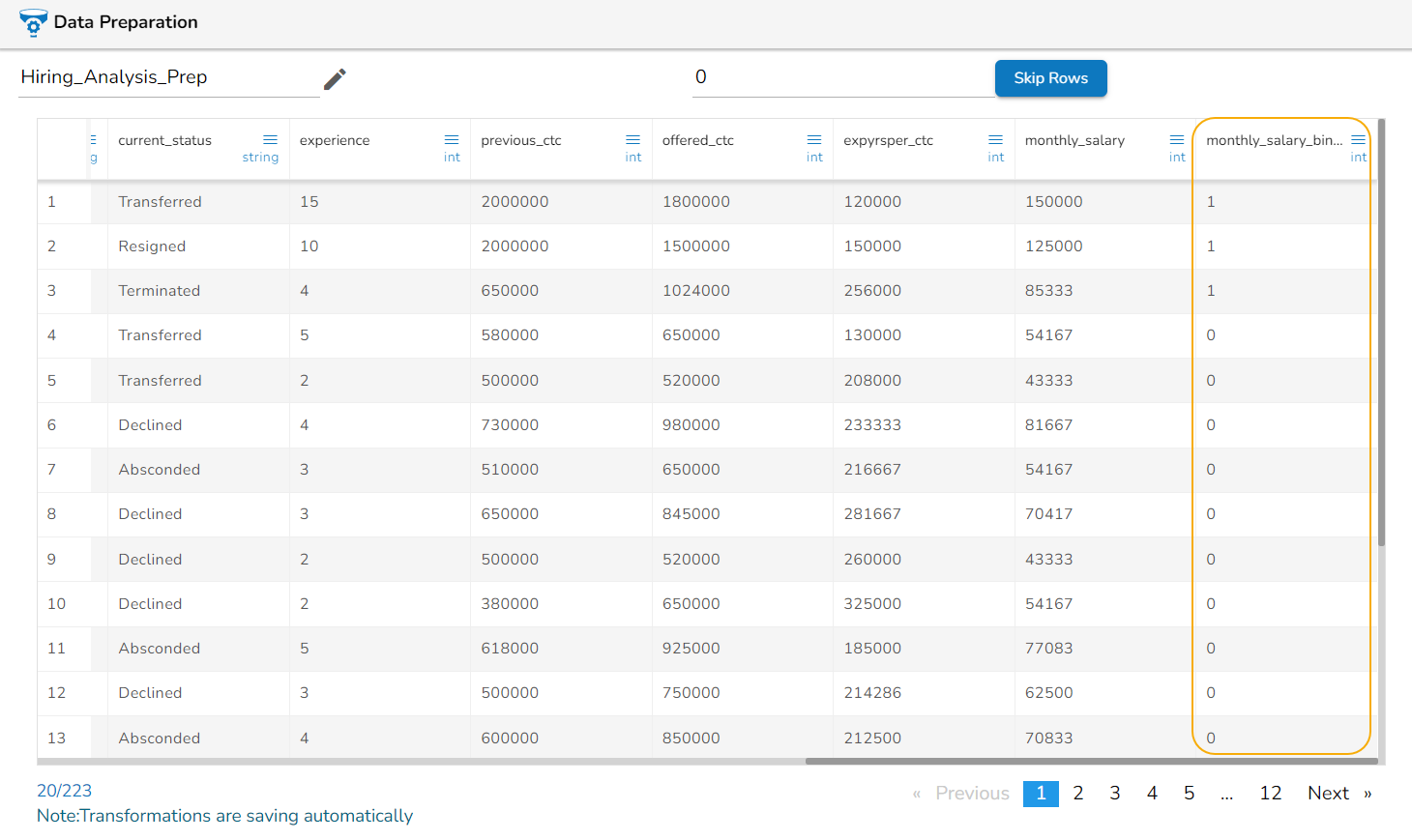
The Dataset gets a new column with the 1 and 0 values by comparing the actual values with the set threshold limit.
Binning/ Discretize values
Binning, also known as discretization, involves converting continuous data into distinct categories or values. This is commonly done to simplify data analysis, create histogram bins, or prepare data for certain machine learning algorithms. Here are the steps to perform this transformation:
Select a Column: Choose the column containing the continuous data that you want to bin.
Select the Transform: Decide on the method of binning or discretization. This could include equal-width binning, equal-frequency binning, or custom binning based on domain knowledge.

Update the Number of Bin Size: Specify the number of bins or categories you want to create from the continuous data using the Binning/ Discretize values dialog box.
Submit It: Execute the binning process with the chosen column and specified number of bins by clicking the Submit option.

Result: The result will be new columns representing the binned or discretized values of the original continuous data.
By following these steps, you can effectively transform continuous data into discrete categories for further analysis or use in machine learning algorithms.
E.g., 1,2,3,4,5,6,7,8,9,10
No. of bins : 3
The result would be 0,0,0,0,1,1,1,2,2,2

Expanding Window Transform
Expanding Window Transform is a common technique used in time series analysis and machine learning for feature engineering. It involves creating new features based on rolling statistics or aggregates calculated over expanding windows of historical data. Here are the steps to perform this transformation:
Select a Numeric Column: Choose a column containing numeric (integer or float) data that you want to transform using the expanding window method.
Select the Expanding Window Transform: Choose the Expanding Window transform option from the available transformations.

The Expanding window transform drawer opens.
Select Method (Min, Max, Mean): Decide on the method you want to apply for calculation within the expanding window. Options typically include Minimum (Min), Maximum (Max), and Mean. User can select multiple columns.
Submit It: Execute the expanding window transformation with the chosen column and method(s) by clicking the Submit option.

The output will be generated as follows:
If multiple methods are selected, new columns will be created with names indicating the method used. For example, if three methods are selected for a column named 'col1', the resulting columns will be named 'col1_Expanding_Min', 'col1_Expanding_Max', and 'col1_Expanding_Mean'.
Calculation:
col1_Expanding_Min: Compares each value to the smallest value from the column and updates the result. The minimum value will always be the least value from the column.
col2_Expanding_Max: Compares each value to the first cell (smallest value) and updates it if a higher value is encountered.
col1_Expanding_Mean: Calculates the mean by adding each value to the first cell value and dividing by the number of elements encountered so far in the expanding window.

Feature Agglomeration
The Feature Agglomeration is indeed used in machine learning and dimensionality reduction for combining correlated features into a smaller set of representative features. It's particularly useful when dealing with datasets containing a large number of features, some of which may be redundant or highly correlated with each other.
Here are the steps to perform the transformation:
Navigate to the Data Preparation workspace.
Select the Feature Agglomeration as the transform from the Transforms tab.

The Feature Agglomeration dialog opens.
Choose multiple numerical columns from your dataset.

Update the samples if needed.
Click the Submit option.

The output will contain the transformed features, where the number of resulting columns will be equal to the number of clusters specified or determined by the algorithm.
Each column will represent a cluster, which is a combination of the original features. The clusters are formed based on the similarity or correlation between features.
If the selected numerical columns are 3 and the sample size is 2, the resulting output will have 2 columns labeled as cluster_1 and cluster_2, respectively, representing the two clusters obtained from the Feature Agglomeration transformation.

Label Encoding
The Label Encoding is a technique used to convert categorical columns into numerical ones, enabling them to be utilized by machine learning models that only accept numerical data. It's a crucial pre-processing step in many machine learning projects.
Here are the steps to perform Label Encoding:
Select a column containing string or categorical data from the Data Grid display using the Data Preparation workspace.
Choose the Label Encoding transform.

After applying the Label Encoding transform, as a result, a new column will be created where the categorical values are replaced with numerical values.
These numerical values are typically assigned in ascending order starting from 0. Each unique category in the original column is mapped to a unique numerical value.
For example:
If a column contains categories "Tall", "Medium", "Short", and "Tall", after applying Label Encoding, it will show the result as 0, 1, 2, 0, respectively. Each unique category gets a distinct numerical value assigned to it based on its position in the encoding scheme.

Lag Transform
The lag transformation involves shifting or delaying a time series by a certain number of time units (lags). This transformation is commonly used in time series analysis to study patterns, trends, or dependencies over time.
Here are the steps to perform a lag transformation:
Navigate to the Data Preparation workspace.
Select the Lag Transform from the Transforms tab.

The Lag Transform dialog box opens.
Choose the numeric-based column representing the time series data.
Update the Lag parameter to specify the number of time units to shift or delay the time series. Provide a number to the Lag field. The Lag value should be 1 or more.
Click the Submit option to submit the transformation.

After applying the lag transformation, the result will be updated with a new column.
This new column represents the original time series data shifted by the specified lag.
The first few cells in the new column will be empty as they correspond to the lag period specified.
The subsequent cells will contain the values of the original time series data shifted accordingly.
For example, if we have a simple time series data representing the monthly sales of a product over a year with a lag of 2, the first two cells in the new column will be empty, and the subsequent cells will contain the sales data shifted by two months.
Month
Sales
Sales_lag_2
Jan
100
Feb
120
Mar
90
100
April
60
120
May
178
90
June
298
60

Leave One Out Encoding
The Leave One Out Encoding transform is to encode categorical variables in a dataset based on the target variable while avoiding data leakage. It's particularly useful for classification tasks where you want to encode categorical variables without introducing bias or overfitting to the training data.
Here are the steps to perform Leave One Out Encoding transformation:
Select a string column for which the transformation is applied. This column should contain categorical variables.
Choose the Leave One Out Encoding transformation from the Transforms tab.

The Leave One Out Encoding dialog box appears.
Select an integer column which represents the target value used to calculate the mean for category values. This column is usually associated with the target variable in your dataset.
Submit the transformation by using the Submit option.

After applying the Leave One Out Encoding transformation, the result will be displayed as a new column.
This new column will contain the mean values of the occurrences for each record in the selected categorical column, excluding the target value in that record.
This encoding method helps to encode categorical variables based on the target variable while avoiding data leakage, making it particularly useful for classification tasks where you want to encode categorical variables without introducing bias or overfitting to the training data. Refer the following image as an example:
category
target
Result
A
1
0.5
B
0
0.5
A
1
0.5
B
1
0
A
0
1
B
0
0.5

Convert Value to Column (One Hot Encoding)
One-Hot Encoding/ Convert Value to Column is a data preparation technique used to convert categorical variables into a binary format, making them suitable for machine learning algorithms that require numerical input. It creates binary columns for each category in the original data, where each column represents one category and has a value of 1 if the category is present in the original data and 0 otherwise.
Here are the steps to perform One-Hot Encoding:
Select Categorical Column: Choose the categorical column(s) from your dataset that you want to encode. These columns typically contain string or categorical values.
Apply One-Hot Encoding: Use the One-Hot Encoding transformation to convert the selected categorical column(s) into a binary format. By clicking the One-Hot Encoding transform, it gets applied to the values of the selected categorical column.

Result Interpretation: The output will be a set of new binary columns, each representing a category in the original categorical column. For each row in the dataset, the value in the corresponding binary column will be 1 if the category is present in that row, and 0 otherwise.
Example: Suppose you have a dataset with a categorical column "Color" containing the following values: "Red", "Blue", "Green", and "Red".
Original Dataset:
Color
Red
Blue
Green
Red
After applying One-Hot Encoding:
Each row represents a category from the original column, and the presence of that category is indicated by a value of 1 in the corresponding binary column. For instance, the first row has "Red" in the original column, hence "Color_Red" is 1, while the others are 0. Like wise "Color_Blue" and "Color_Green" are displayed.
1
0
0
0
1
0
0
0
1
1
0
0

Principal Component Analysis
Principal Component Analysis (PCA) is a dimensionality reduction technique used to identify patterns in data by expressing the data in a new set of orthogonal (uncorrelated) variables called principal components. The PCA is widely used in various fields such as data analysis, pattern recognition, and machine learning.
Here are the steps to perform Principal Component Analysis (PCA):
Navigate to the Data Preparation workspace.
Select the Principal Component Analysis transform using the Transforms tab.

The Principal Component Analysis dialog window opens.
Select multiple numerical columns by using the given checkboxes.

The selected columns get displayed separated by commas.
Output Features: Update output features by providing a number based on the number provided for this field, the result columns are inserted in the data set.
Click the Submit option.

Here's an illustration to explain the Principal Component Analysis:
Suppose we have a dataset with two numerical variables, "Height" and "Weight", and we want to perform PCA on this dataset.
Original Dataset:
170
65
165
60
180
70
160
55
After standardization:
0.44
0.50
-0.22
-0.50
1.33
1.00
-1.56
-1.00
Based on the provided update output features, the result column(s) get added.

Please Note: The selected Output Feature for the chosen dataset is 1, therefore in the above given image one column has been inserted displaying the result values.
Rolling Data
The Rolling Data transform is used in time series analysis and feature engineering. It involves creating new features by applying transformations to rolling windows of the original data. These rolling windows move through the time series data, and at each step, summary statistics or other transformations are calculated within the window.
Here are the steps to perform the Rolling Data transform:
Select a numeric (int/ float) based column from your dataset. This column represents the time series data on which you want to apply the Rolling Data transformation.
Select the Rolling Data transform.

Update the Window size. Specify the size of the rolling window. This determines the number of consecutive data points included in each window. The window size should be a numeric value of 1 or larger number.
Select a Method out of the given choices (Min, Max, Mean). It is possible to choose all the available methods and apply them on the selected column.

Click the Submit option to apply the rolling window transformation.

Please Note: Window Size can be updated by any numeric values which must be 1 or larger values.
The result will be the creation of new columns based on the selected method and the specified window size. Each new column will contain the summary statistic or transformation calculated within the rolling window as it moves through the time series data.
For Example: Suppose we have a time series dataset with a numeric column named "Value" containing the following values: [1, 2, 3, 4, 5, 6, 7, 8, 9, 10], and we want to apply a rolling window transformation with a window size of 2 and calculate the Min, Max, and Mean within each window.
In this example, each new column represents the summary statistic (Min, Max, or Mean) calculated within the rolling window of size 2 as it moves through the "Value" column.
The Result Columns:
"Value_Min": [null, 1, 2, 3, 4, 5, 6, 7, 8, 9]
"Value_Max": [null, 2, 3, 4, 5, 6, 7, 8, 9, 10]
"Value_Mean": [null, 1.5, 2.5, 3.5, 4.5, 5.5, 6.5, 7.5, 8.5, 9.5]

Please Note: The first cell in each new column is null because there are no previous cells to calculate the summary statistic within the initial window.
Singular Value Decomposition
The Singular Value Decomposition transform is a powerful linear algebra technique that decomposes a matrix into three other matrices, which can be useful for various tasks, including data compression, noise reduction, and feature extraction. In the context of transformations for data analysis, Singular Value Decomposition (SVD) can be used as a technique for dimensionality reduction or feature extraction. It works by breaking down a matrix into three constituent matrices, representing the original data in a lower-dimensional space.
Here are the steps to perform the Singular Value Decomposition transform:
Select the Singular Value Decomposition transform using the Transforms tab.

The Singular Value Decomposition window opens.
Select multiple numeric types of columns from the dataset using the drop-down menu.
Update the Latent Factors.
Click the Submit option.

The result should be based on the latent factor update size. For example, if it's 2 the result column will be 2.

Target-based Quantile Encoding
Target-based Quantile Encoding is particularly useful for regression problems where the target variable is continuous. It helps in encoding categorical variables based in a dataset based on the distribution of the target variable within each category which can potentially improve the predictive performance of regression models.
Here are the steps to perform the Target-based Quantile Encoding transform:
Select a string column from the dataset on which the Target-based Quantile Encoding can be applied.
Select the Target-based Quantile Encoding transformation from the Transforms tab.

The target-based quantile encoding dialog box opens.
Select an integer column from the dataset.
Click the Submit option.

The result will be a new encoded column for each value in the selected column.
E.g.,
category
target
Result
A
1
0.875
B
0
0.125
A
1
0.875
B
1
0.125
A
0
0.875
B
0
0.125

Target encoding
Target Encoding, also known as Mean Encoding or Likelihood Encoding, is a method used to encode categorical variables based on the target variable(or another summary statistic) for each category. It replaces categorical values with the mean of the target variable for each category. This encoding method is widely used in predictive modeling tasks, especially in classification problems, to convert categorical variables into a numerical format that can be used as input to machine learning algorithms.
Here are the steps to perform the Target Encoding transform:
Select a category (string) column type for the transformation.
Select the Target Encoding transformation from the Transforms tab.

The Target Encoding dialog box opens.
Select the Target Column using the drop-down option (it should be numeric/integer column).
Click the Submit option.

The result will be displayed in a new column with the encoded mean values for each category value in the selected column will be displayed.

E.g.,
Category
Target
Result
A
1
0.5257
B
0
0.4247
A
1
0.5257
B
1
0.4247
A
0
0.5257
B
0
0.4247
Weight of Evidence Encoding
The Weight of Evidence Encoding is used in binary classification problems to encode categorical variables based on their predictive power to the target variable. It measures the strength of the relationship between a categorical variable and the target variable by examining the distribution of the target variable across different categories.
Here are the steps to perform the Weight of Evidence Encoding transform:
Select a categorical column (string column) from the dataset.
Select the Weight of evidence encoding transform from the Transforms tab.

Select a target column with Binary Variables (like true/false, 0/1). E.g., the selected column in this case, is the target_value column.
Click the Submit option.

The result will be as new column where the distribution of the target variable across different categories.

Last updated