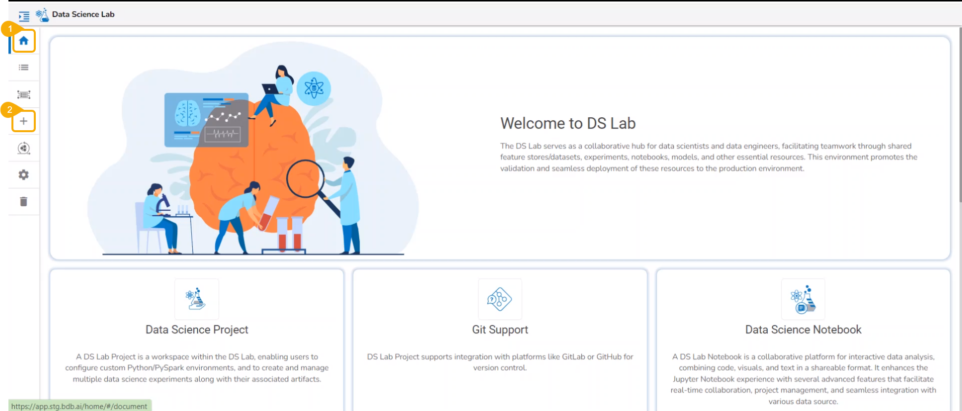
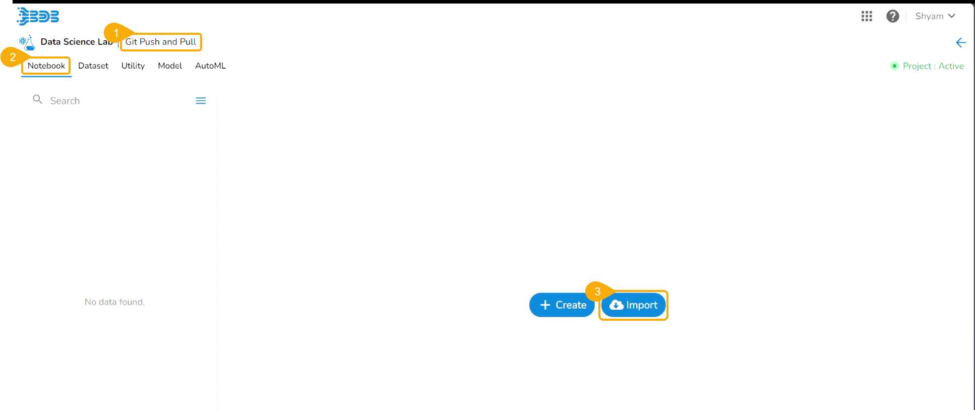
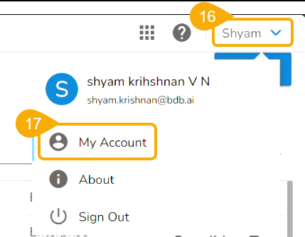
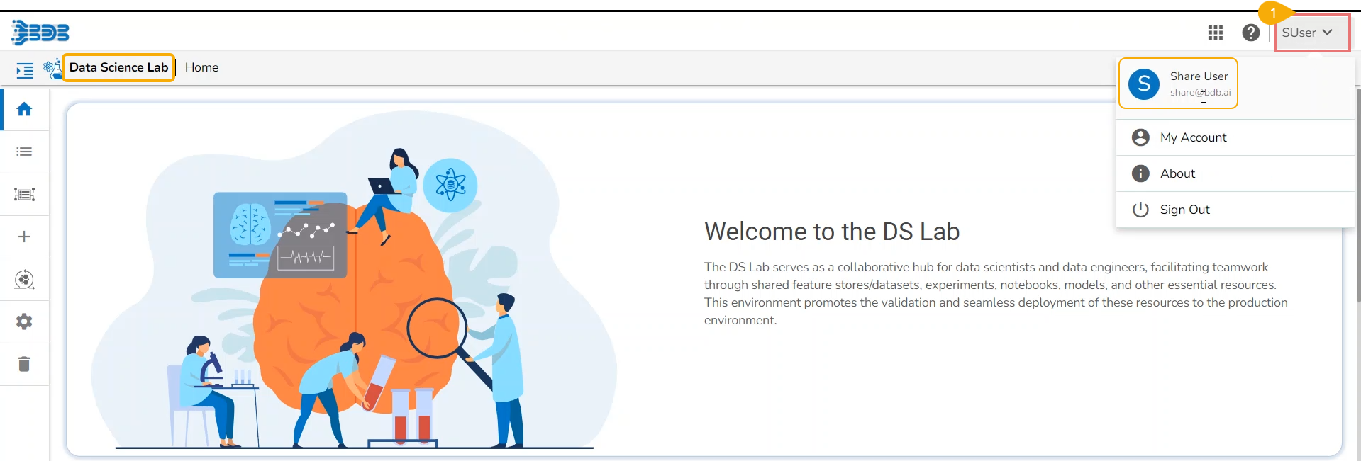
This page displays the steps to access the DS Lab module under the platform.
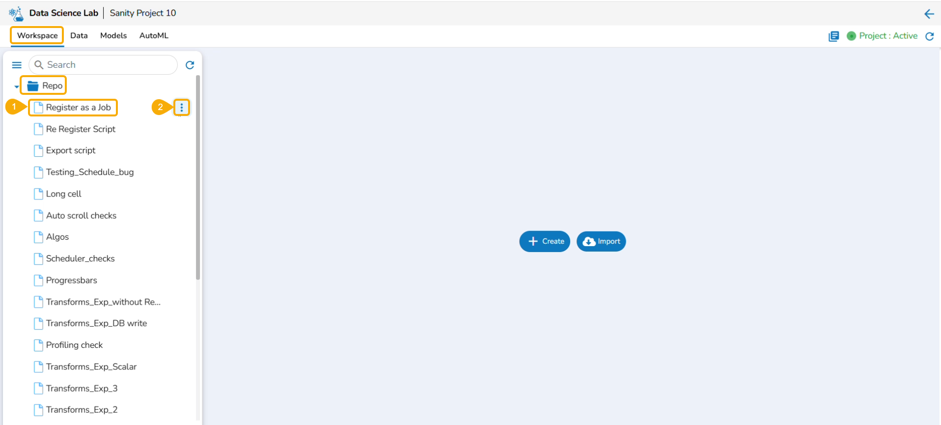
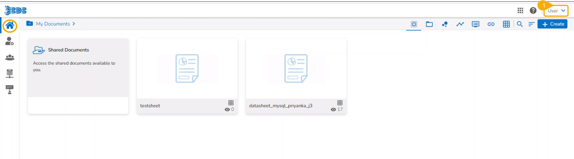
Navigate to the Platform Homepage.
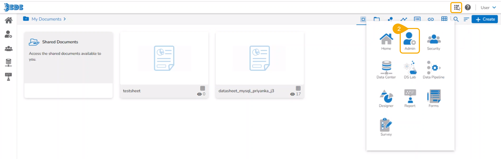
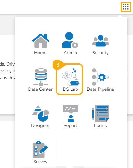
Click the Apps menu icon on the Platform homepage.
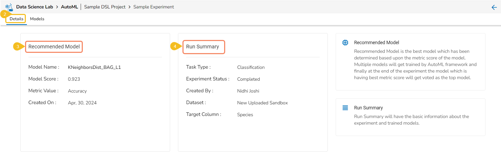
Click the DS Lab module.
The user gets redirected to the Homepage of the Data Science Lab module.
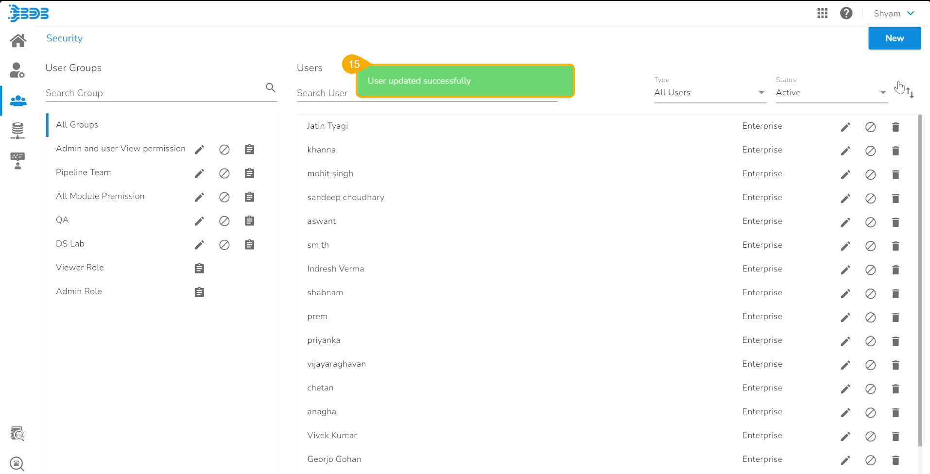
Please Note: To access the DS Lab module available inside the Apps menu, the logged-in user must have the to access it from the security level settings.
What is Data Science Lab?
The BDB Data Science Lab serves as a collaborative hub for data scientists to work together. Within this module, they can collectively conduct experiments, and exchange Notebooks, models, and other important elements with their team. This collaborative environment allows for validation and seamless deployment of these resources to the Production environment.
What is a Data Science Project?
A Data Science Project created inside the Data Science Lab is like a Workspace inside which the user can create and store multiple data science experiments and their associated artifacts.
Please Note:
The user can create a new Notebook for coding or upload an existing Notebook only after Activating a Data Science Project.
What is a Feature Store?
A Feature Store is a centralized repository for storing, managing, and serving features used in machine learning models. It plays a crucial role in the machine learning lifecycle by providing a consistent and efficient way to manage features. It is a scalable solution for organizing and cataloging features, making them easily accessible to data scientists and ML engineers across an organization.
Feature Stores facilitate collaboration, version control, and reusability of features, streamlining the ML development process and improving model quality and efficiency.
What is a Workspace?
A Workspace in a Data Science module provides a cohesive and integrated environment that supports the end-to-end data science workflow, from data ingestion and processing to analysis, model building, and deployment.
The Workspace is a placeholder to create and save various data science experiments inside the Data Science Lab module.
The Workspace is the default tab to open for each Data Science Lab project.
What is a Notebook/ Data Science Notebook?
A Data Science Notebook is an interactive and collaborative digital platform used by data scientists and analysts for data exploration, analysis, modeling, and visualization. It combines executable code, visualizations, and explanatory text in a flexible and shareable format, making it a versatile tool for data science projects. Key features include code execution, rich text and visualizations, interactive data exploration, collaboration and sharing, reproducibility and documentation, and integration with data science libraries and tools.
In the current Data Science Lab module a .ipynb file that is created or imported inside a project works like a Data Science Notebook for the users. The Workspace tab of a Data Science Project contains such Data Science Notebooks in a Repo folder.
What is Data Set in context to Data Science Lab module?
A dataset in data science is a structured collection of data used for analysis and modeling. It represents a specific domain or problem and can include various data types. Datasets are essential for tasks like data analysis, modeling, and extracting insights in both supervised and unsupervised learning. They can be sourced from different domains and collected from surveys, experiments, or existing databases. Datasets contain features and labels for supervised learning, while they are unlabeled for unsupervised learning. They are typically split into training and test sets. Publicly available datasets are widely used for research and benchmarking. Datasets form the foundation for various data science tasks and enable solving complex problems.
The Data Set tab provided under the Data Science Lab module supports the following types of Data sets:
Dataset - Here, Dataset stands for a table or filtered data from database.
Data Sandbox - Data Sandbox are files that are uploaded or appended to Data Sandbox folder from local directory (excel, csv, text etc.).
What is a Data Science Model?
A data science model refers to a mathematical or computational representation of a real-world phenomenon or problem that data scientists use to make predictions, gain insights, or automate decision-making processes. It is a key component of the data science workflow and is built using data, statistical techniques, and algorithms.
The Model tab under a Data Science Project includes:
Imported Models: Models trained using external tools and libraries, which are brought into the data science workflow for analysis or prediction tasks.
Models created in Data Science Lab Notebook: Models built and trained within the Data Science Lab Notebook environment, utilizing its features and capabilities.
AutoML Models: Models generated through automated machine learning (AutoML) techniques, which automatically search and select the best model based on the given data and desired outcome.
What is Utility script?
The Utility tab allows to create and list the python scripts (.py files) that can be imported to your notebook.
What is AutoML?
AutoML (Automated Machine Learning) refers to the automated process of building and optimizing machine learning models without extensive manual intervention. It leverages intelligent algorithms and techniques to automate tasks such as data preprocessing, feature selection, model selection, hyperparameter tuning, and model evaluation. AutoML aims to simplify and accelerate the model development process, enabling users with limited machine learning expertise to create effective models efficiently.
The Auto ML tab allows the users to create data science experiments and lists them.
Create
This section displays steps on how to create a Project or Feature Store.
Working with the Workspace tab
This section explains way to begin work with the Workspace tab. The Create and Import options are provided for Repo folders.
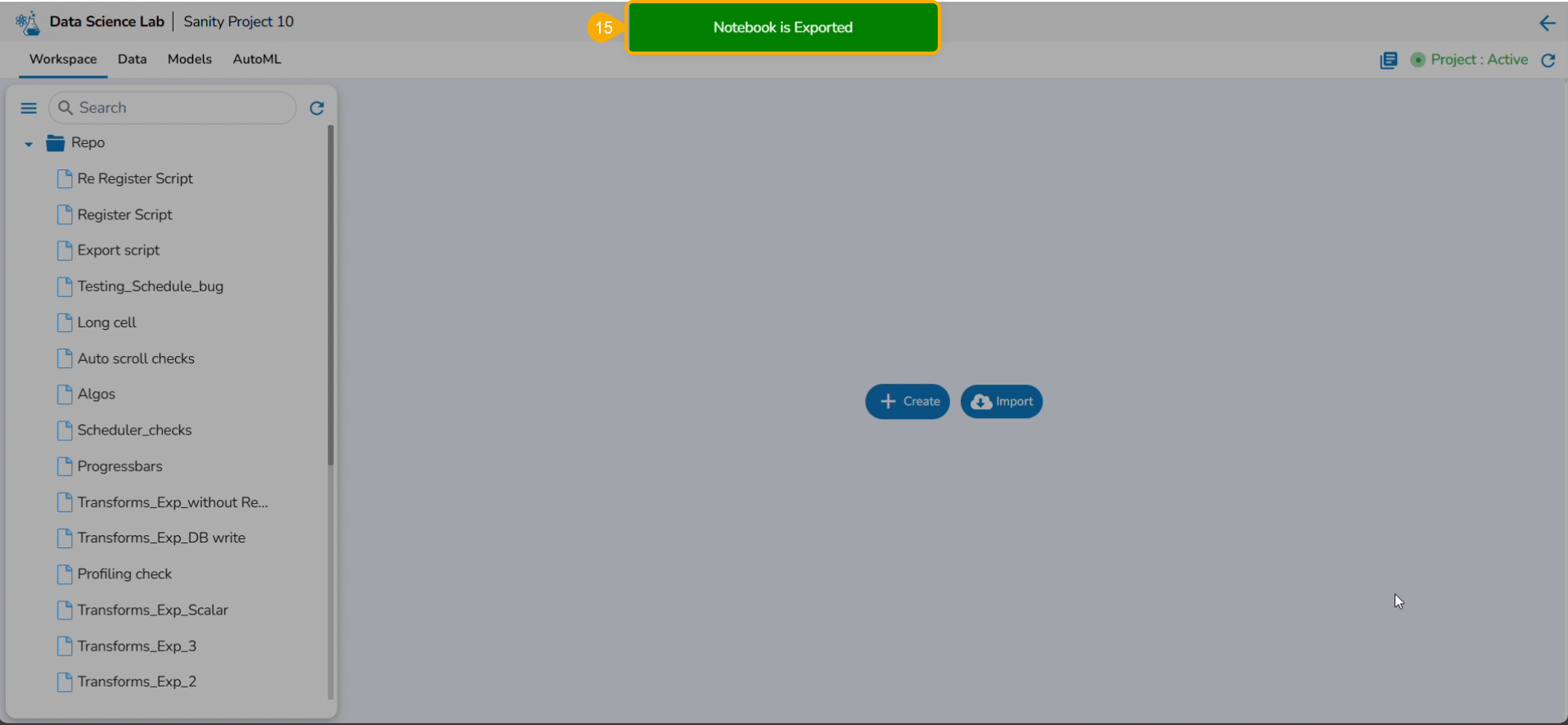
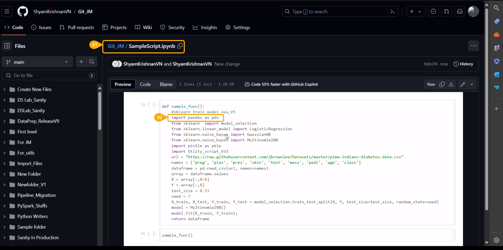
This page displays the steps to Export a DSL script and register it as Job.
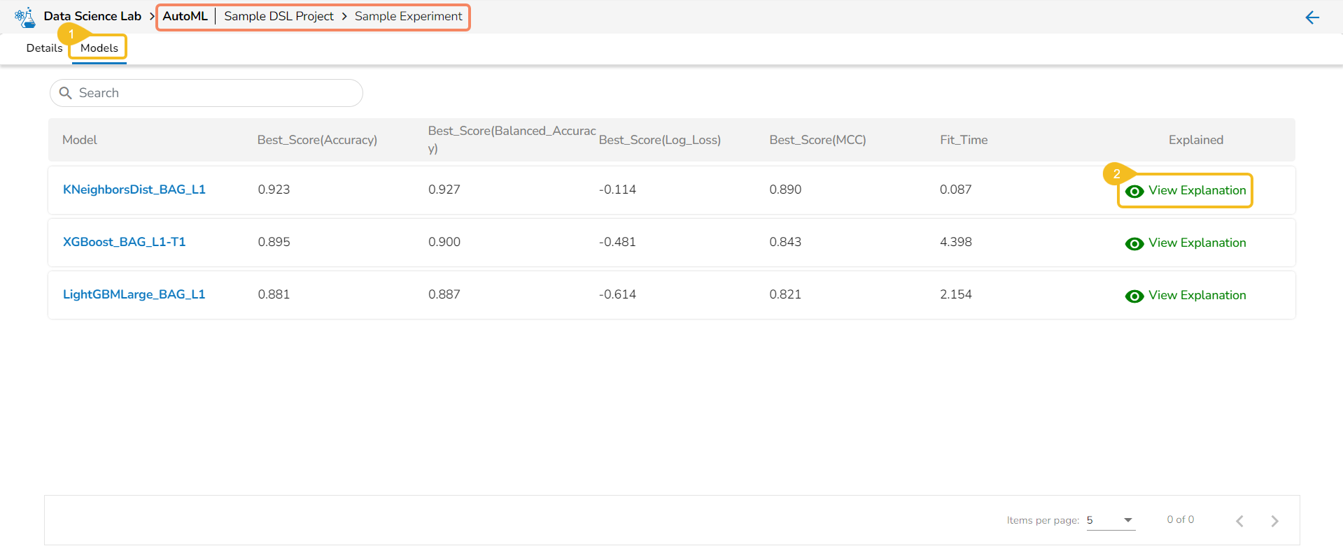
View Explanation
The View Explanation option will redirect the user to the below given options. Let us see all of them one by one explained as separate topics.
Data Science Notebook
Explore the page where all the Data Science activities take place. The listed topics will be supported only for .ipynb files.
Notebook Actions
The credited options provided to a Notebook are explained under this section.
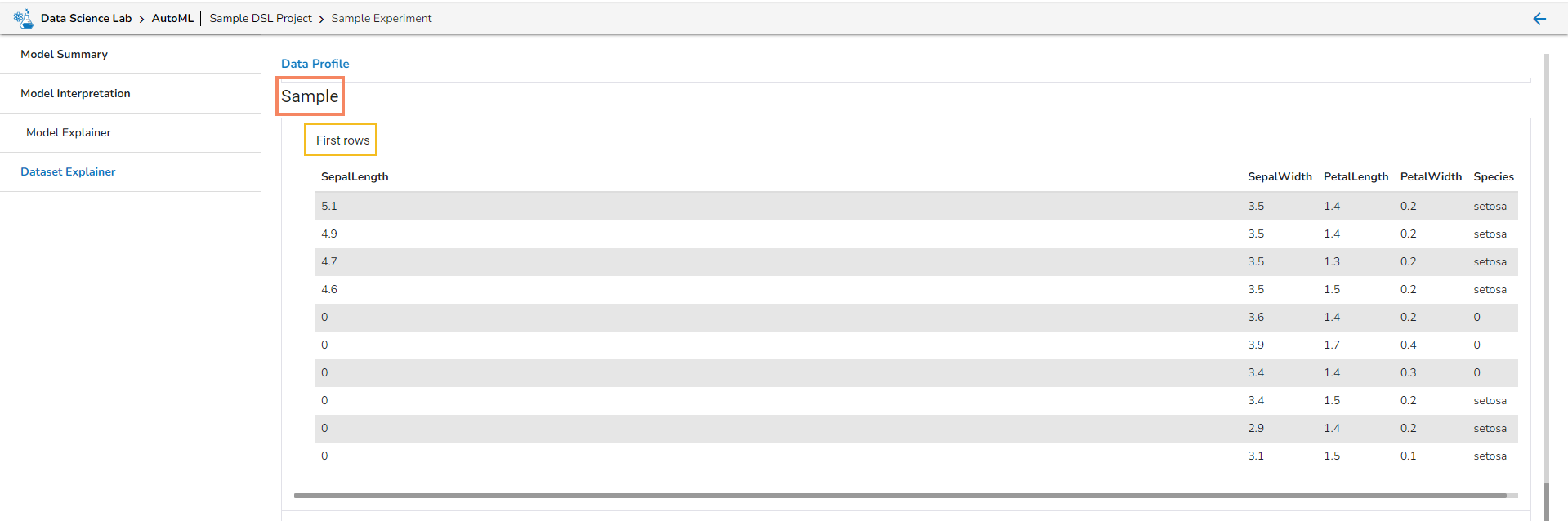
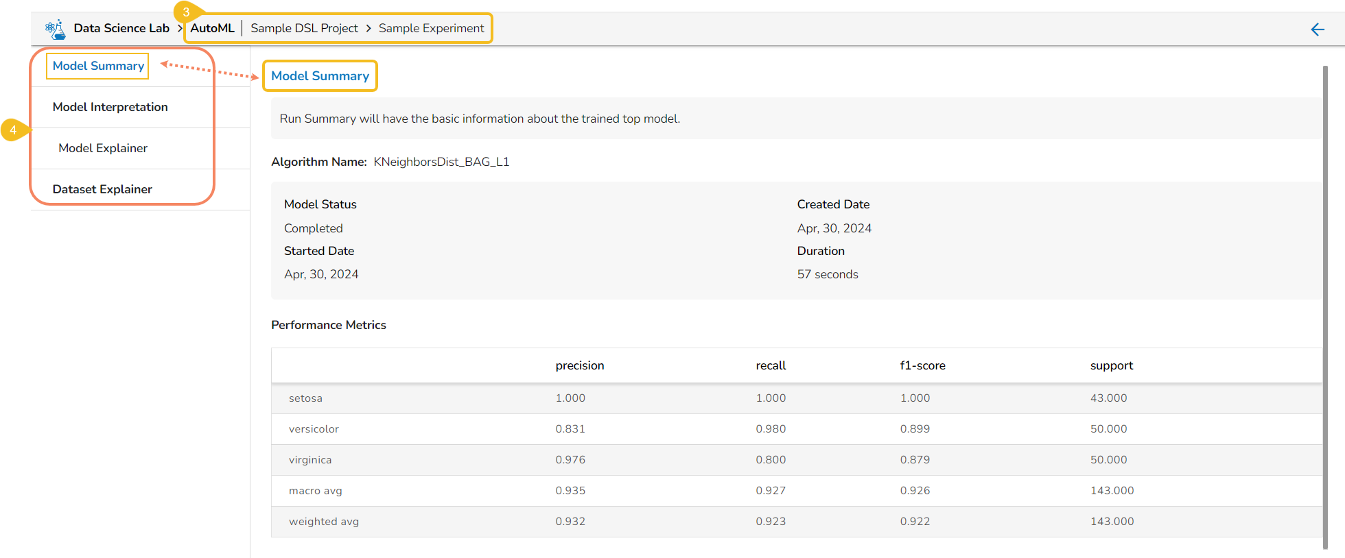
Model Interpretation
The user is taken to a dashboard upon clicking Model Explainer to gather insights and explanations about predictions made by the selected AutoML model.
Model interpretation techniques like SHAP values, permutation importance, and partial dependence plots are essential for understanding how a model arrives at its predictions. They shed light on which features are most influential and how they contribute to each prediction, offering transparency and insights into model behavior. These methods also help detect biases and errors, making machine learning models more trustworthy and interpretable to stakeholders. By leveraging model explainers, organizations can ensure that their AI systems are accountable and aligned with their goals and values.
Please Note:The user can access the Model Explainer Dashboard under the Model Interpretation pageonly.
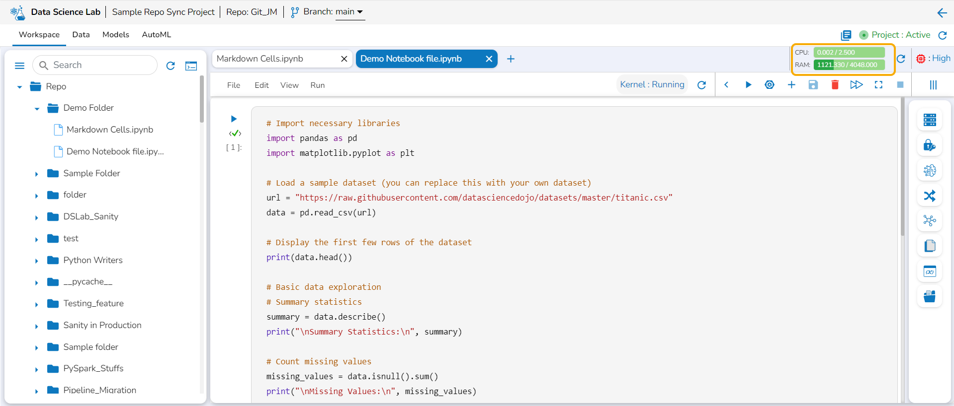
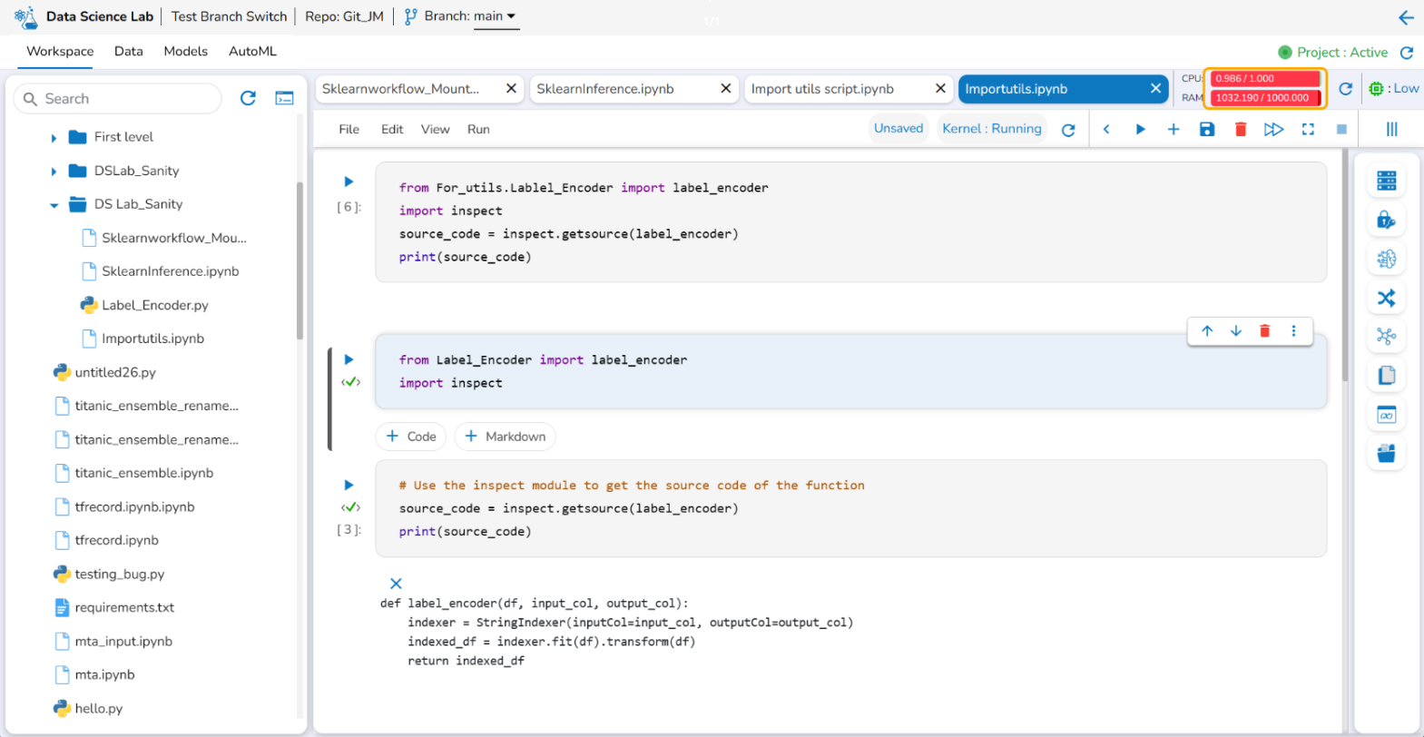
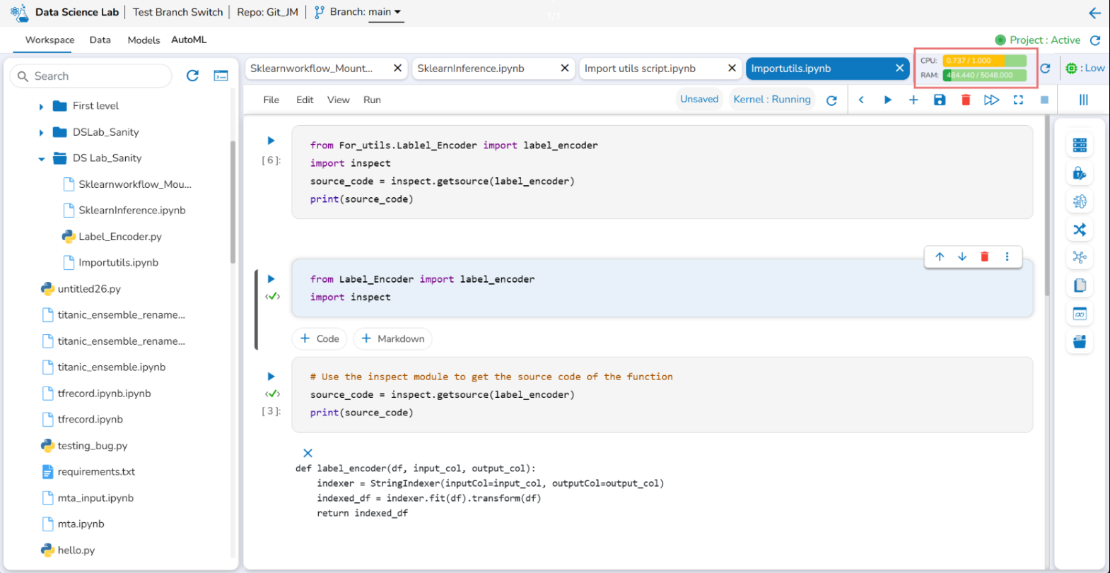
Container Status Message
A DSL Project displays various status of the container on the top right side of the header panel.
The user gets all the updates regarding container status through color coded message display for a specific DSL Project. After creating a new project and opening it the user gets to see various status messages on the top right side of the page.
Steps to see the container message:
Open an active Data Science Project.
The user gets redirected to create or import Notebook.
The container status message gets displayed on the top right side of this screen.
The following status messages get displayed till the container gets created and comes into the running status.
Please Note: A container status message appears when container is not available. An error message also appears to inform user that the Project container is not up and running.
Container status message when container is getting created, and it is initializing.
Container status message when container is running.
Please Note: The user can click on the branch icon to get the latest branch related configuration.
Settings
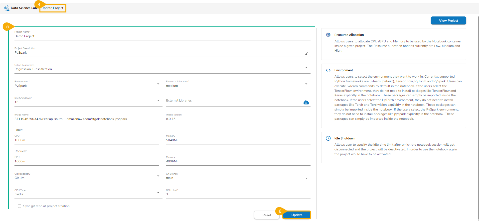
This page helps the user to access and modify the default settings for the DSL Project.
Check out the given illustration on how to access and save modifications for the Project default settings.
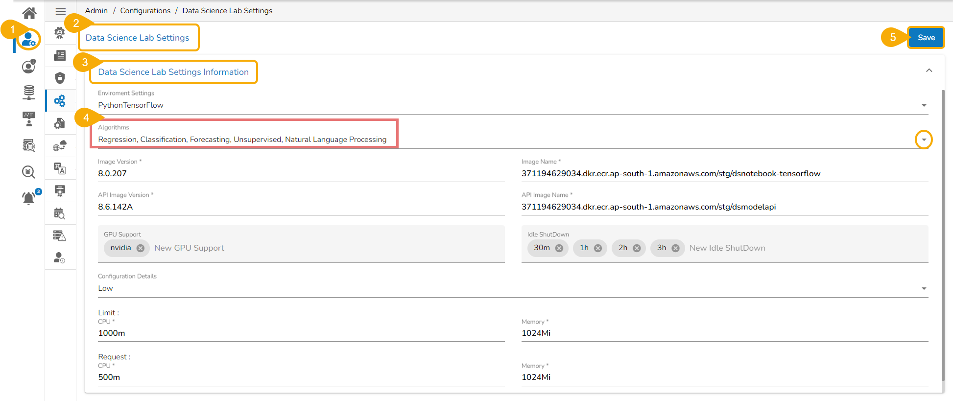
Navigate to the Home page of Data Science Lab module.
The Settings icon appears in the left side menu panel. Click the Settings option.
Click the DefaultSettings page opens displaying the default settings.
The user can modify the following details:
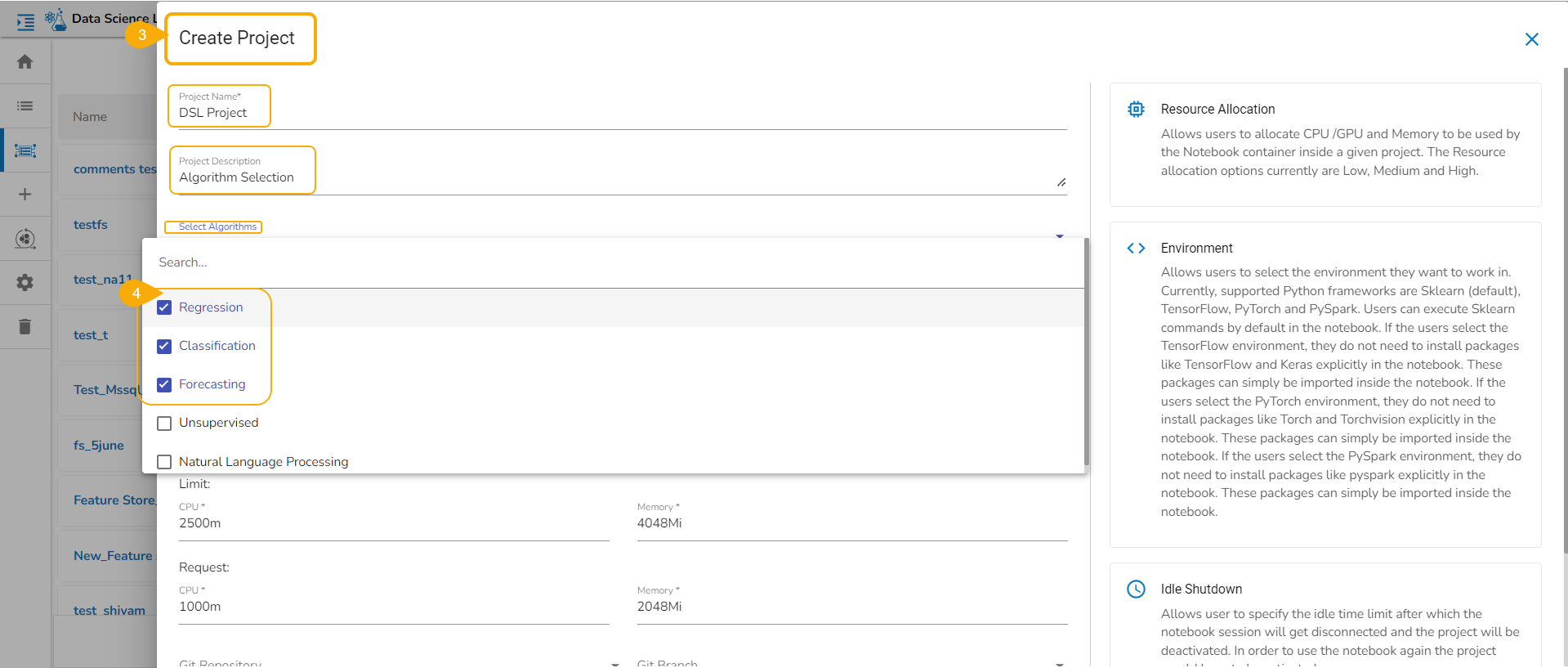
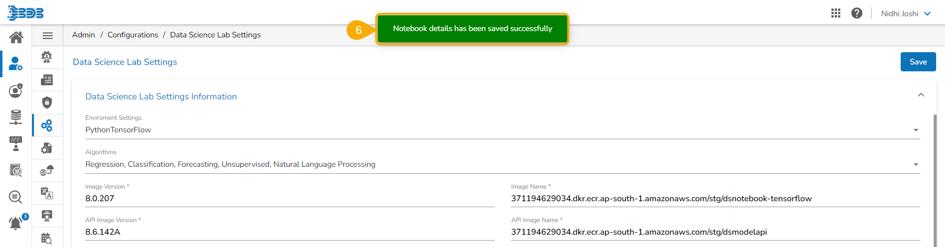
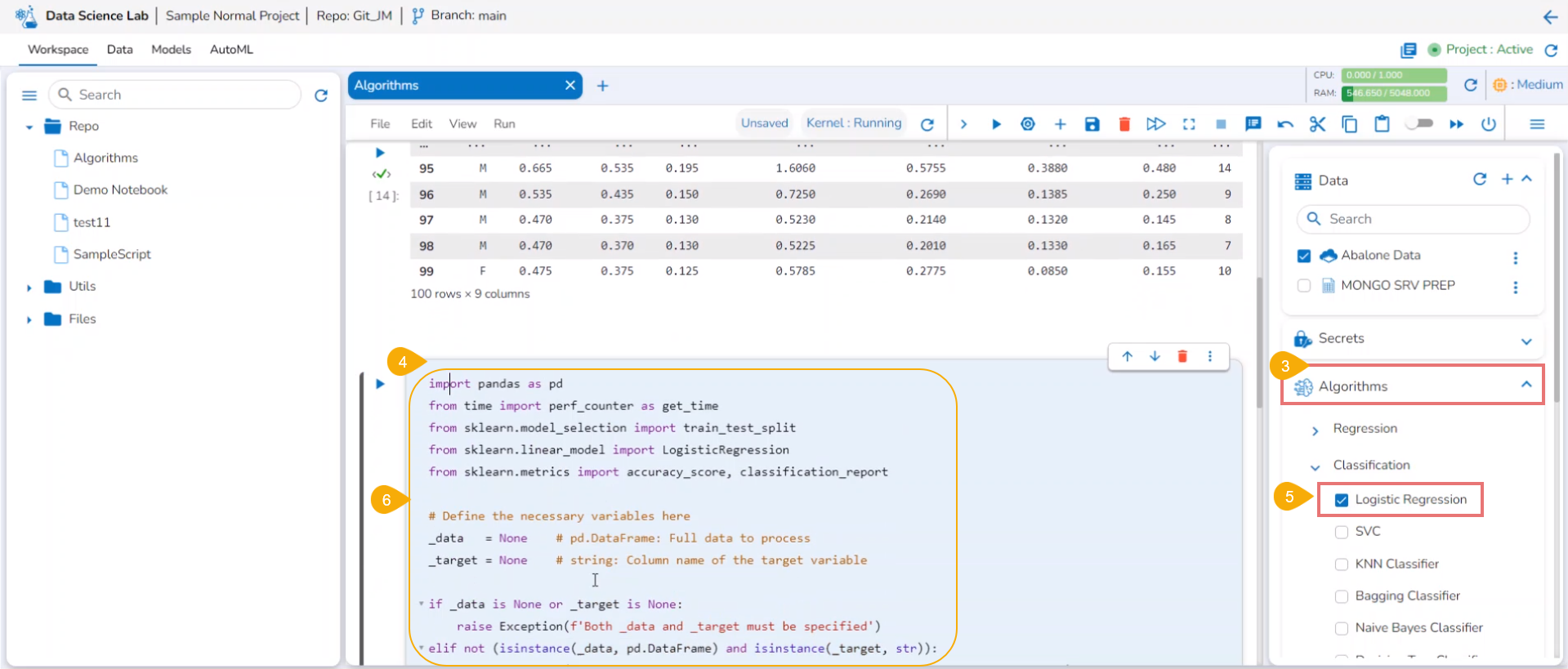
Algorithms: The user can select or deselect algorithms from the given drop-down menu. The provided choices are Regression, Classification, Forecasting, Unsupervised, Natural Language Processing.
A notification message appears and the modified default settings will be saved.
AutoML
The Auto ML tab allows the users to create various experiments on top of their datasets and list all the created experiments.
Automated Machine Learning (AutoML) is a process that involves automating the selection of machine learning models and hyperparameters tuning. It aims to reduce the time and resources required to develop and train accurate models by automating some of the time-consuming and complex tasks.
The Auto ML feature provided under the Data Science Lab is capable of covering all the steps, from starting with a raw data set to creating a ready-to-go machine learning model.
An Auto ML experiment is the application of machine learning algorithms to a dataset.
Please Note:
AutoML functionality is a tool to help speed up the process of developing and training machine learning models. It’s always important to carefully evaluate the performance of a model generated by the AutoML tool.
The Create Experiment option is provided on the .
Homepage
The homepage is a centralized hub where users can access, interact with, and manage the various features, functionalities, and resources provided by the Data Science Lab module.
The users can access the various sections of the Data Science Lab module using the menu on the left side of the homepage.
The following options are provided on the left side menu of the Homepage:
Icon
Name
Action
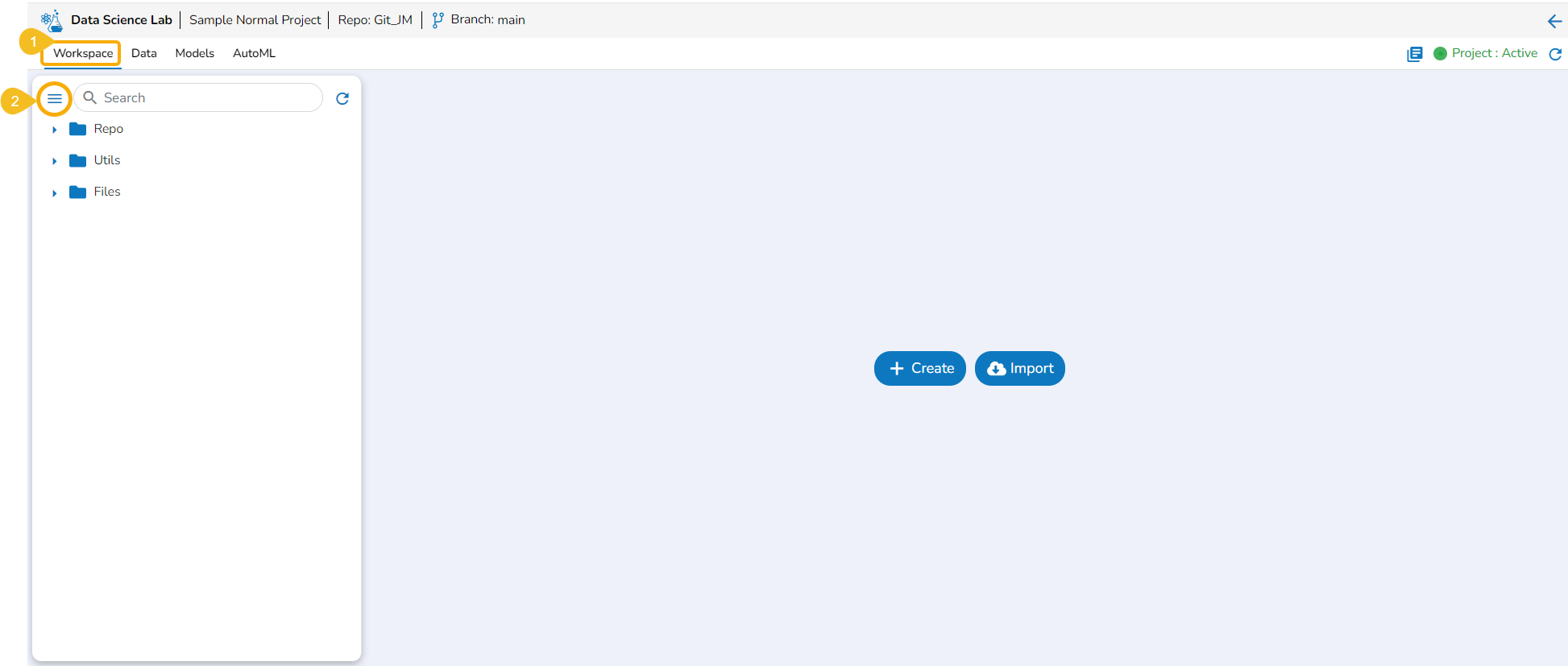
Workspace Folders
The Workspace tab contains default folders named Repo, Utils, and Files. All the created and saved folders and files will be listed under either of these folders.
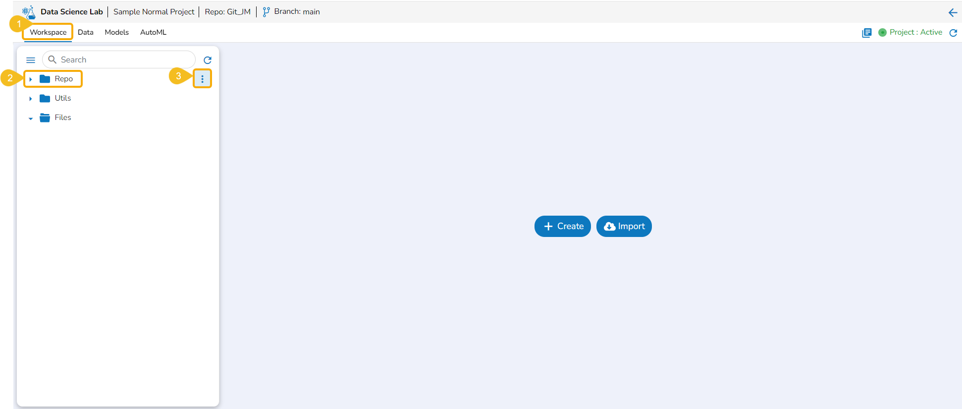
Accessing Workspace Default Folders
Navigate to the Workspace tab (it is a default tab to open for a Project).
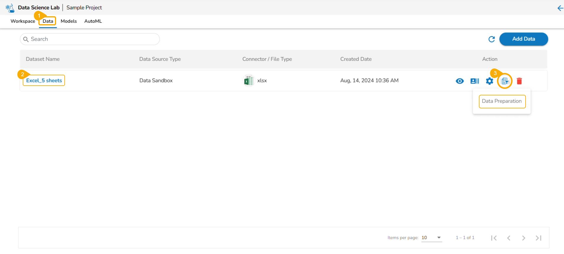
Data
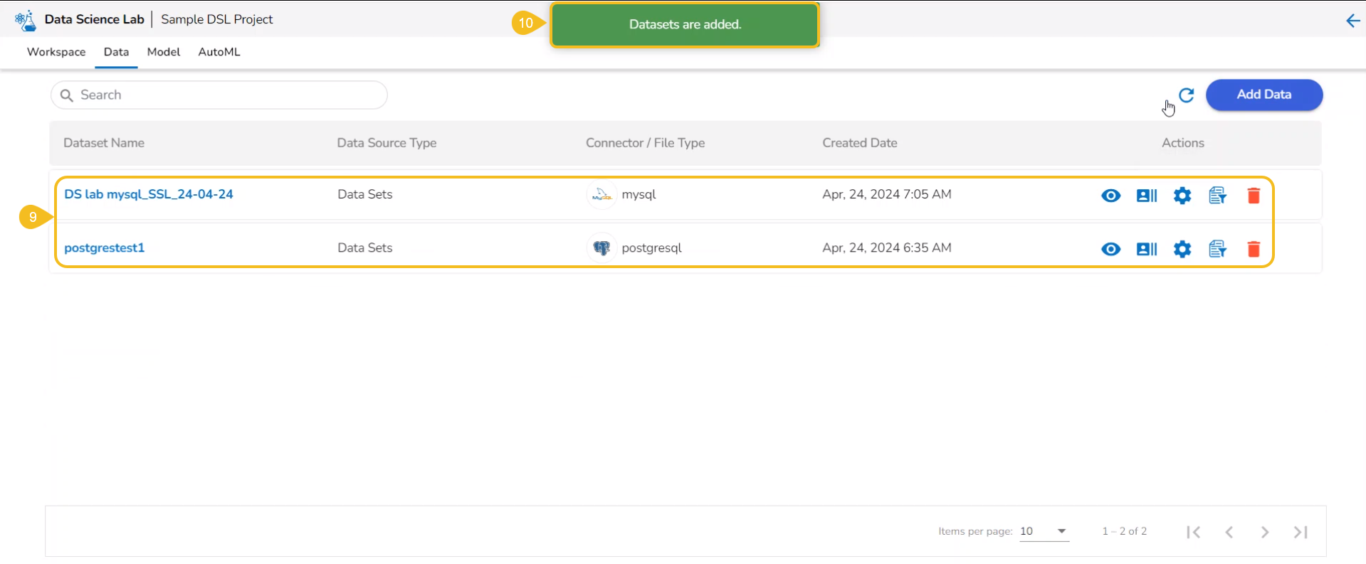
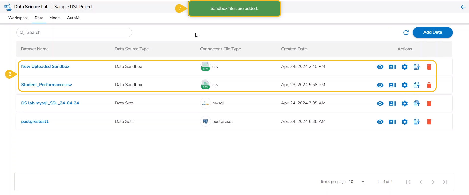
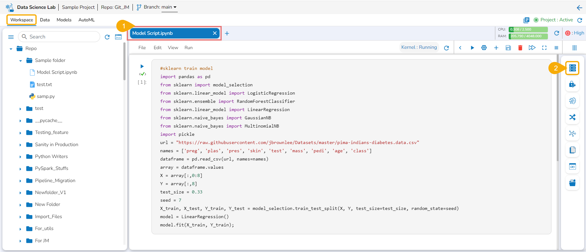
This section focuses on how to add or upload datasets to your DSL Projects. The Dataset tab lists all the added Data to a Project.
The Add Data option provided under the Data tab redirects the users to add various types of data to a DSL Project. The users can also upload sandbox files or create feature stores using this functionality.
Please Note: Users can add Datasets by using the Data tab or Notebook page provided under the Workspace tab.
Files Attributes
This section helps the user to understand the attributes provided to the file folder created inside a normal Data Science Lab project.
Accessing the File Folder Attributes
Check out the illustration to access the attributes for a File folder.
Register a Model
To register a model implies pushing the model into the Pipeline environment where it can be used for inferencing when Production data is read.
Please Note:The currently supported model types are: Sklearn (ML & CV), Keras (ML & CV), and PyTorch (ML).
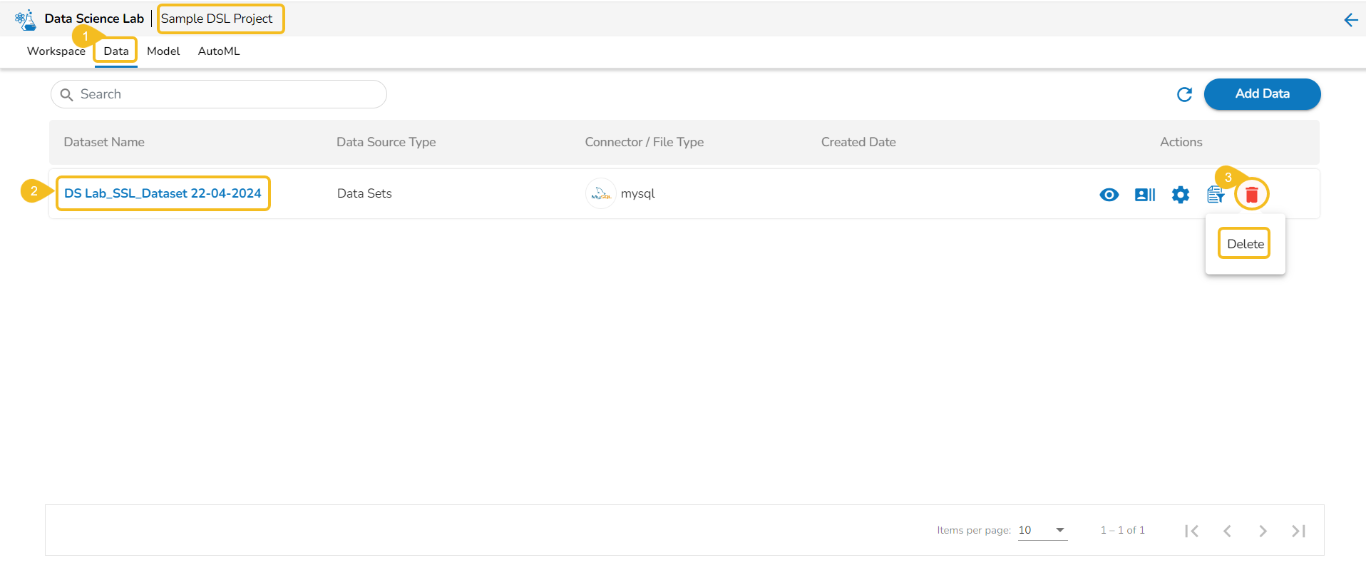
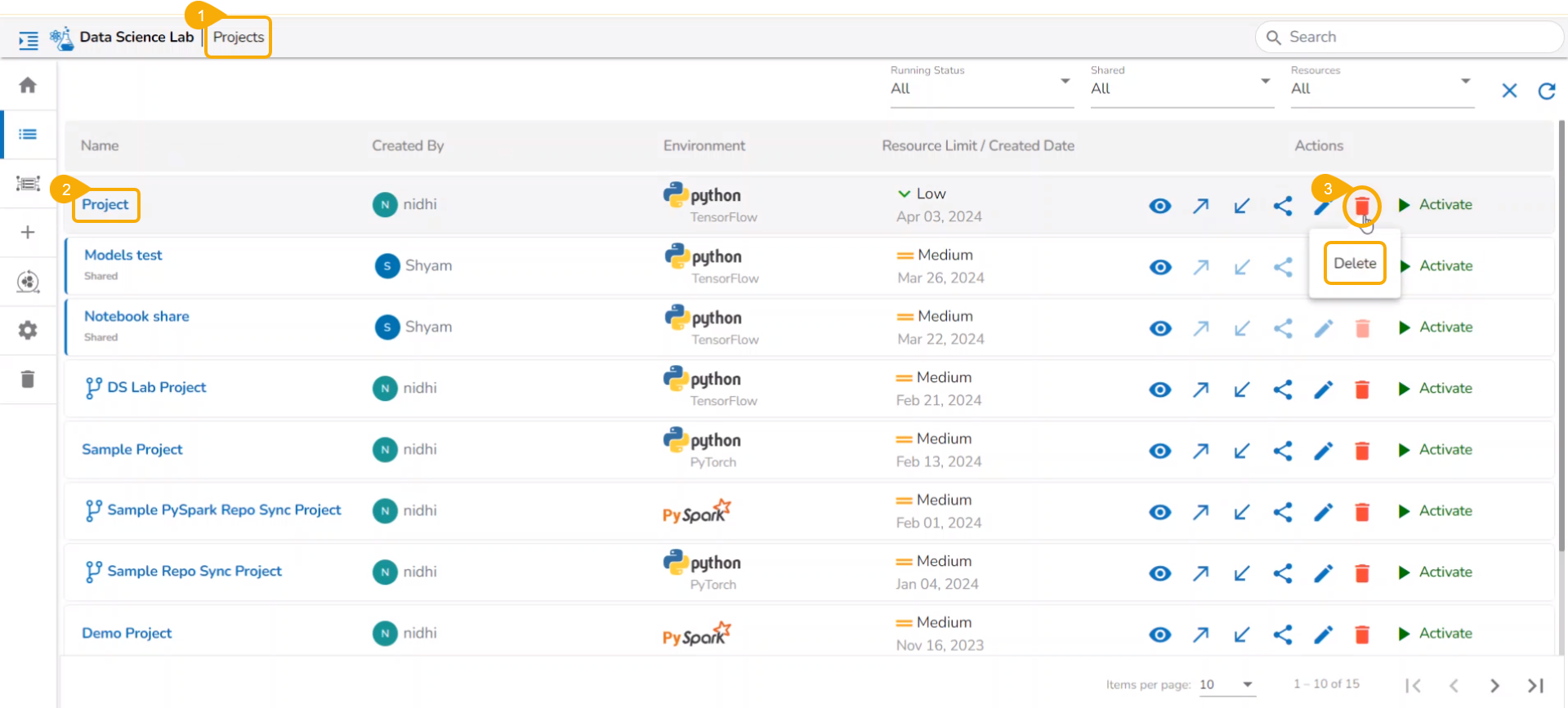
Delete a Model
This section focuses on how to delete a model using the Models tab.
Users can delete any unregistered model using the delete icon from the Actions panel of the Model list.
Check out the illustration on deleting a model.
Navigate to the
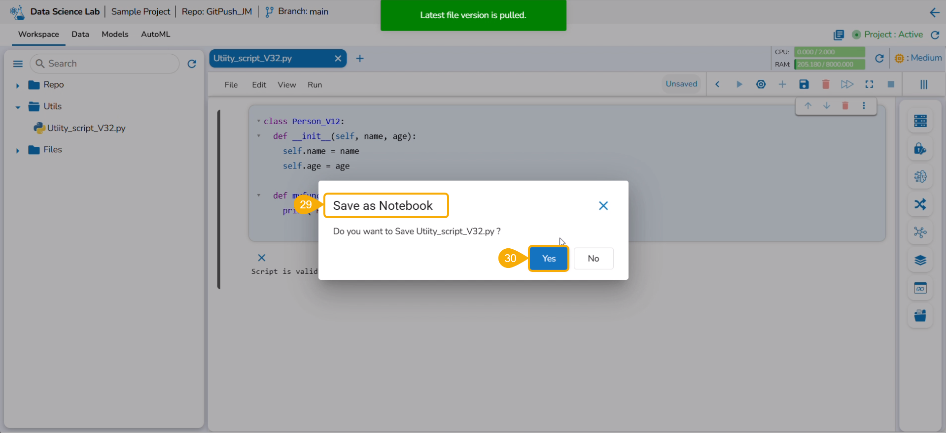
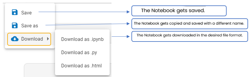
Save as Notebook
This section explains Save as Notebook functionality for the .ipynb files.
A dialog box opens each time to save the recent changes from the user while closing the selected opened .ipynb file at any given time. The user can click the Yes option to save the Notebook.
Navigate to an opened Data Science Notebook (.ipynb file) and modify the notebook content.
Click the Close icon provided to close the Notebook infrastructure.
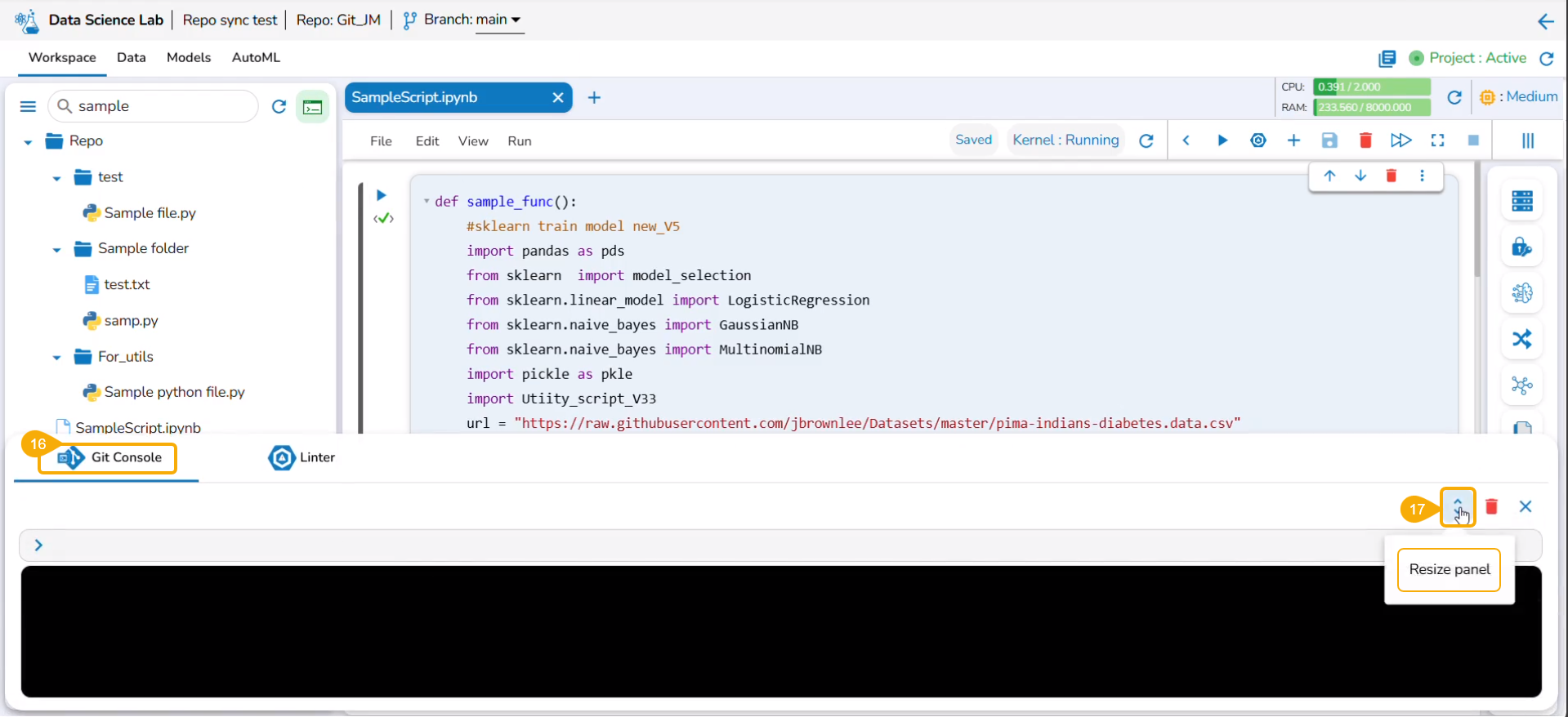
Adjustable Repository Panel
Users can manually adjust the width of the repository panel to sight multiple files and sub-folders.
Users can manually adjust the width of the repository panel in the Workspace tab, allowing for better visibility and organization of multiple sub-folders and files within a project.
Check out the illustration to understand how users can adjust the repository panel inside a DS Project.
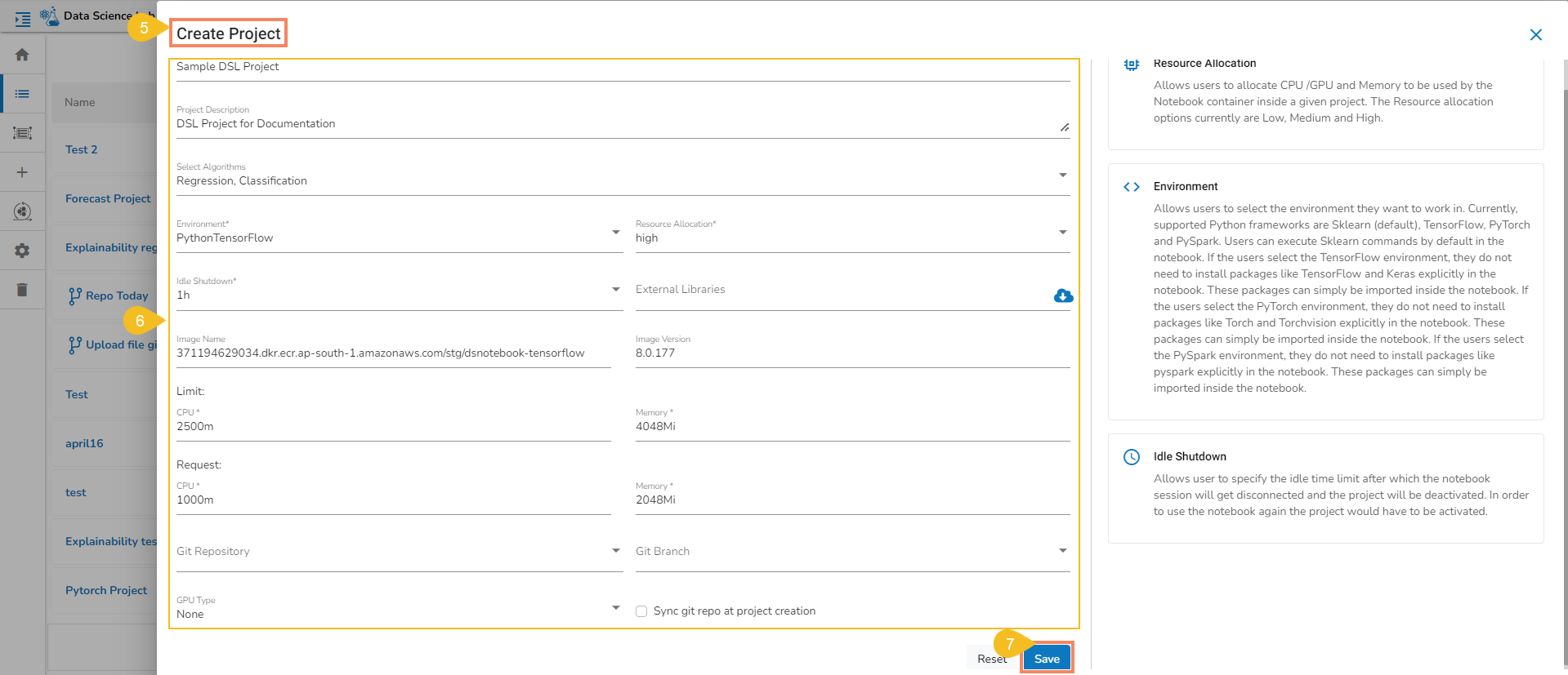
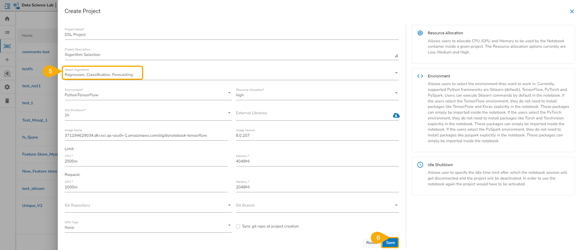
Environment: The user can select an Environment option from the given choices. The provided choices are Python TensorFlow, Python PyTorch, PySpark.
Resource Allocation: The user can select a Resource Allocation option from the given choices. The provided choices are low, medium, and high.
Idle Shutdown: The user can select a time limit option for idle shutdown. The provided time limit options are 30m, 1h, and 2h.
Click the Save option.
Modifying the Default Project Settings
Home
Opens the homepage of the Data Science Lab module.
Redirects to the Project List page.
Redirects to the Feature Store List page.
Left Menu on the DSL Homepage
The left side panel displays the default Folders.
These folders will save all the created or imported folders/ files by the user.
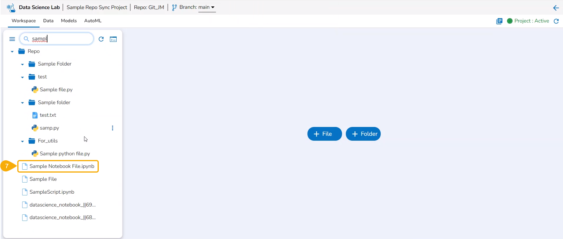
The Workspace tab also contains a Search bar to search the available Assets.
Please Note: The Workspace will be blank for the user, in case of a new Project until the first Notebook is created. It will contain the default folders named Repo, Utils, and Files.
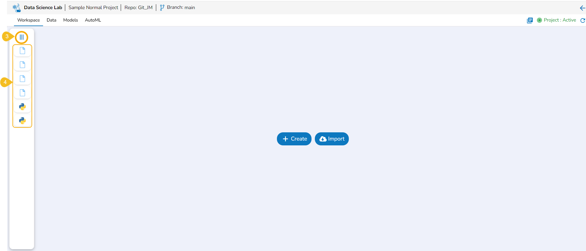
Collapsing the Left side Panel
Navigate to the Workspace Assets.
Click the Collapse icon.
Expanded Notebook List
The Workspace left-side panel will be collapsed displaying all the created or imported files and folders as icons.
Collapsed Notebook List
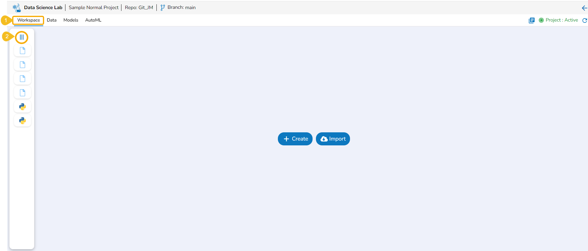
Expanding the Left side Panel
Navigate to the Workspace tab with the collapsed left-side panel.
Click the Expand icon.
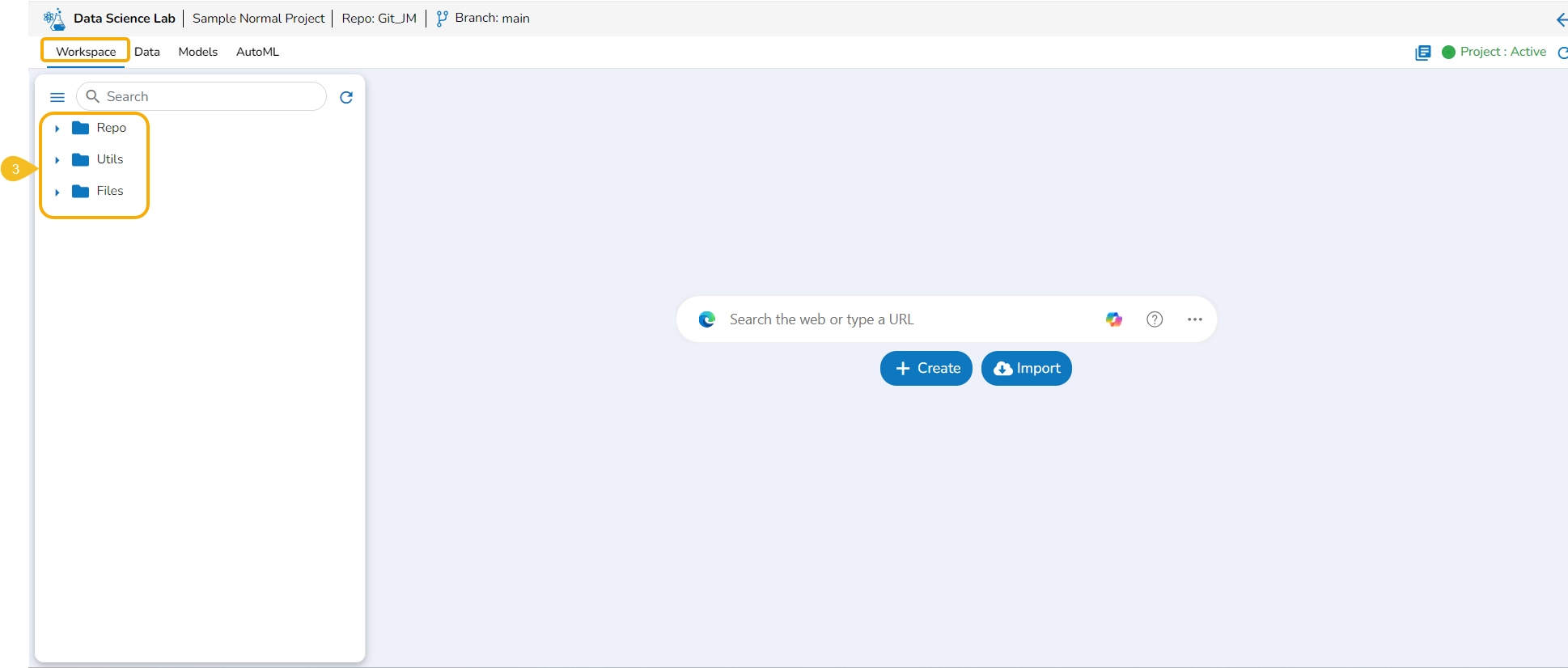
The Workspace's left-side panel will be expanded. In the expanded mode of the left-side panel, the default folders of the Workspace tab will be visible in the default view.
Please Note:
The Workspace left side menu appears in the expanded mode by default while opening the Workspace tab.
The Workspace List displays the saved/ created folders and files in the collapsed mode (if any folder or file is created inside that Workspace).
The normal Data Science Project where Git Repository and Git Branch are selected while creating the project, displays the selected branch on the header.
A Repo Sync Project can display the selected branch on the Project header, and the user will be allowed to change the branch using the drop-down menu.
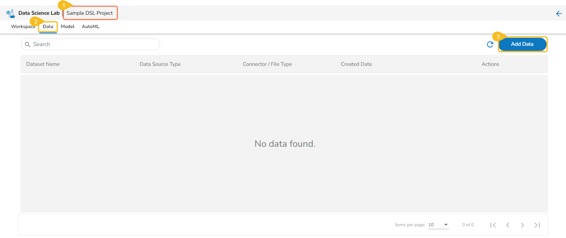
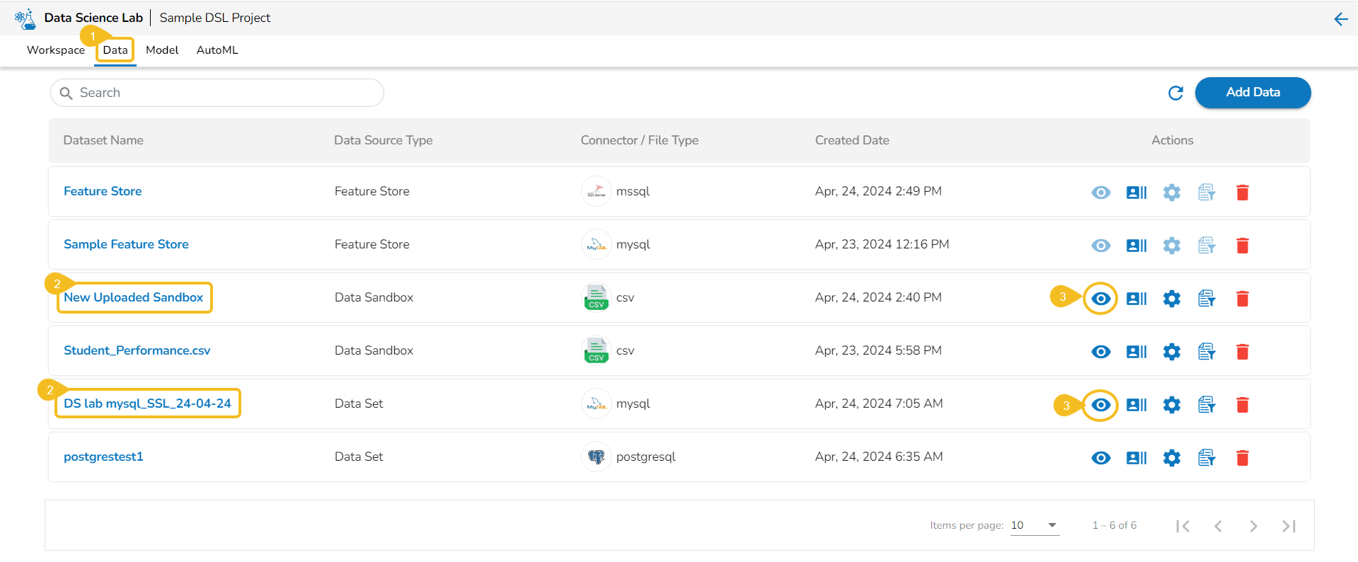
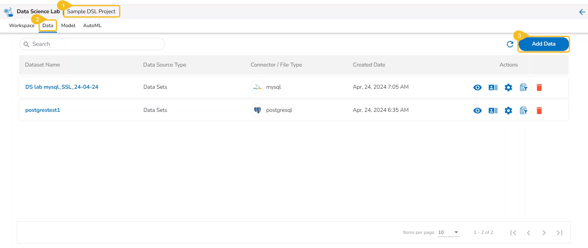
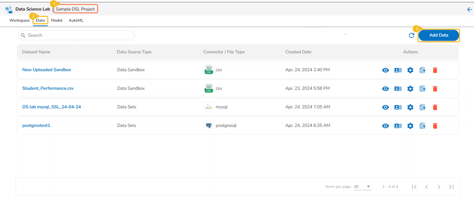
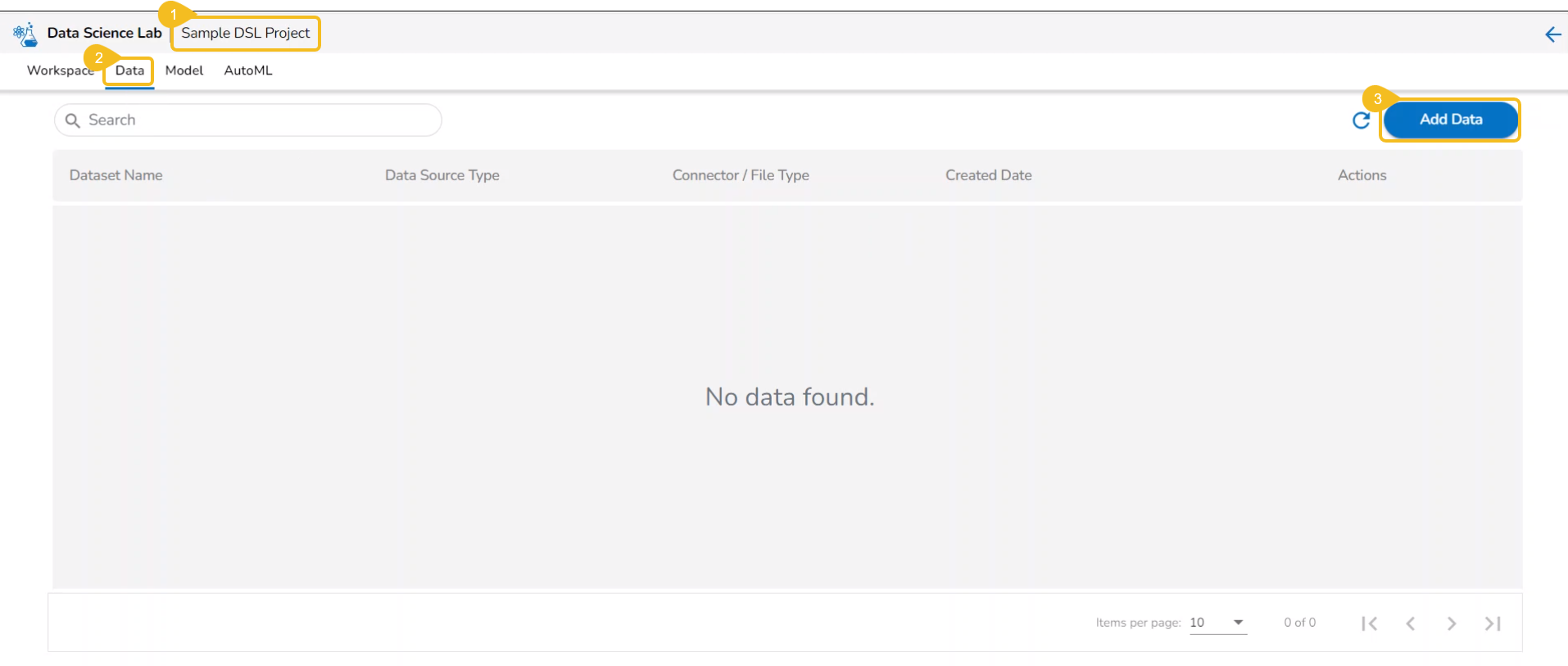
Open a Data Science Lab Project.
Click on the Data tab from the opened Project.
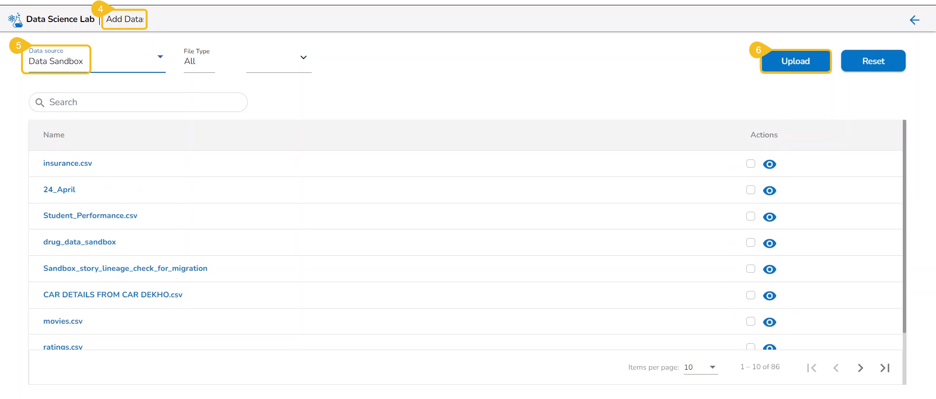
The Data tab opens displaying the Add Data option.
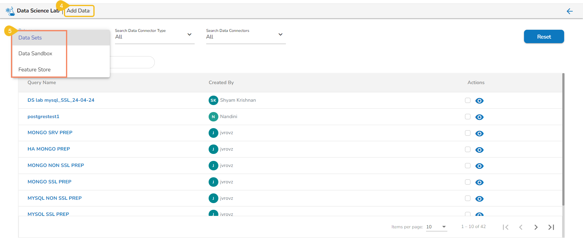
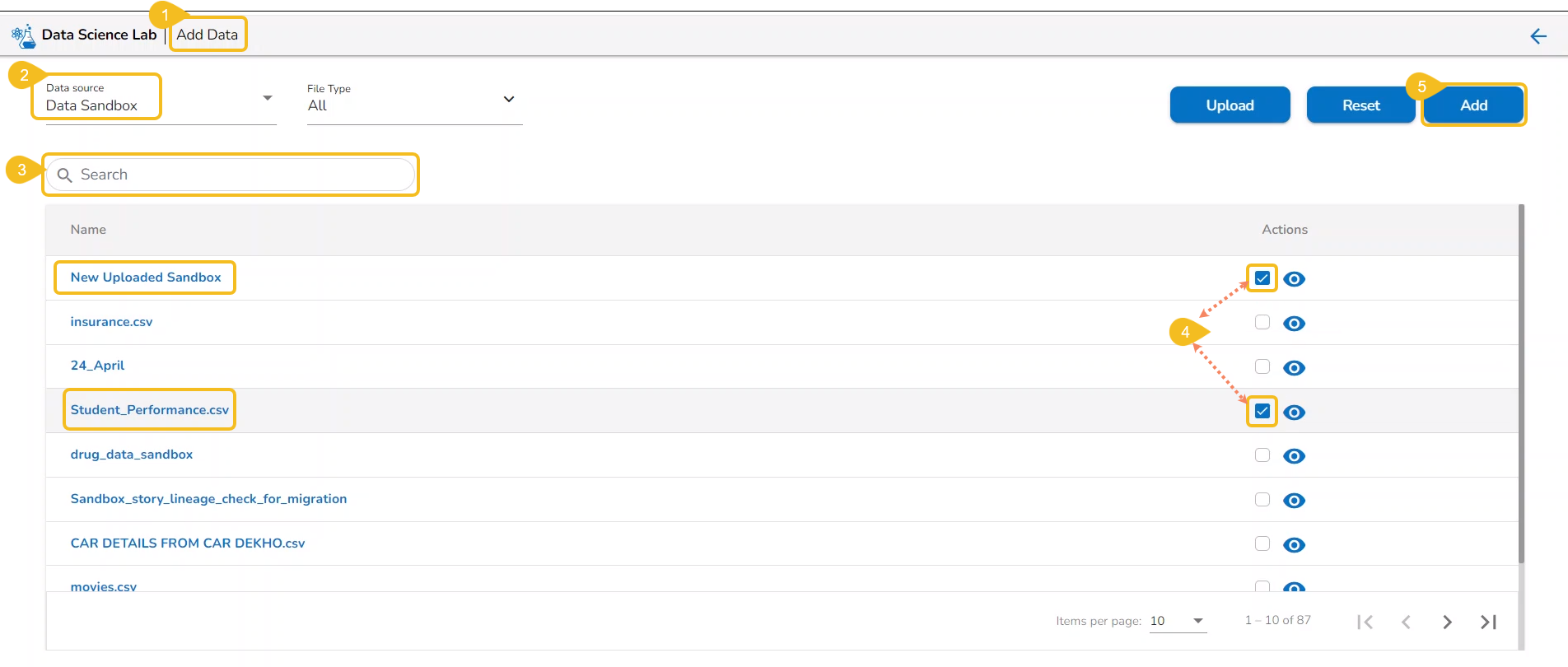
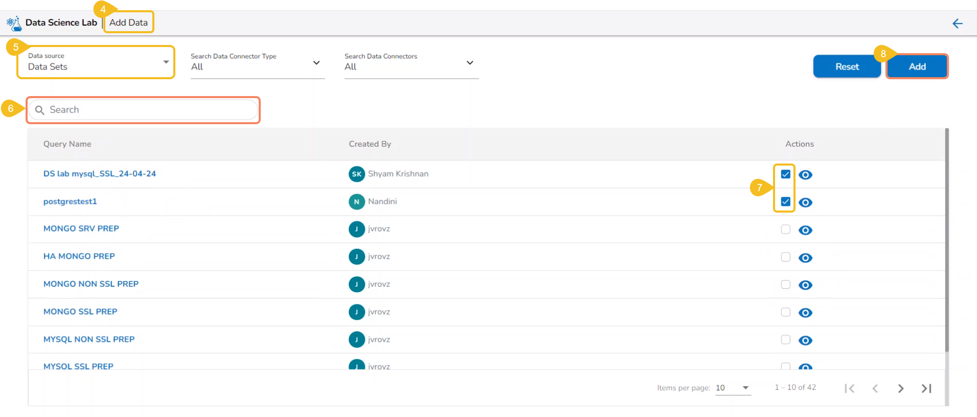
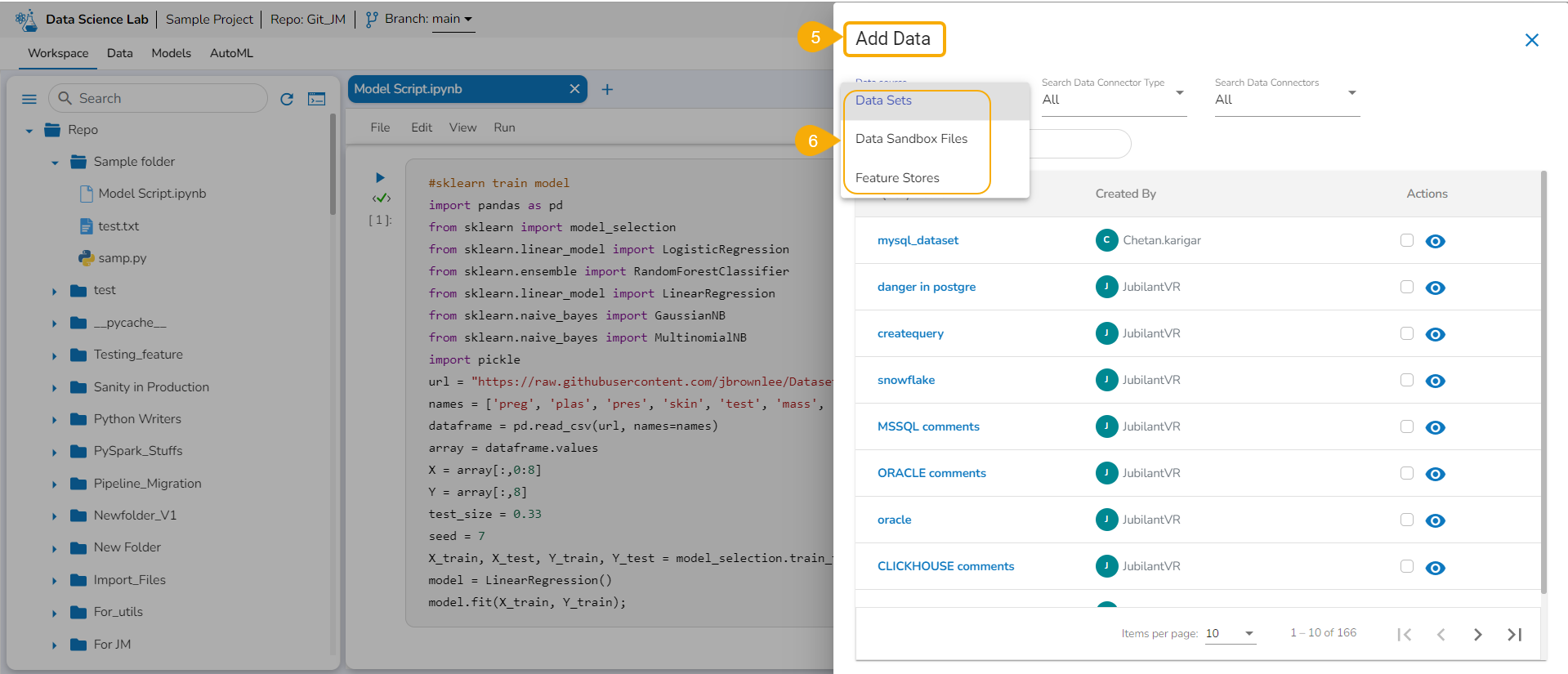
The Add Data page opens the uploaded and added Data Sources for the selected DSL Project.
The Add Data page offers the following Data source options to add as datasets:
Data Sets– These are the uploaded data sets from the Data Center module.
Data Sandbox – This option lists all the available/ uploaded Data Sandbox files.
Feature Store – This option lists all the available Feature Stores under the selected DSL Project.
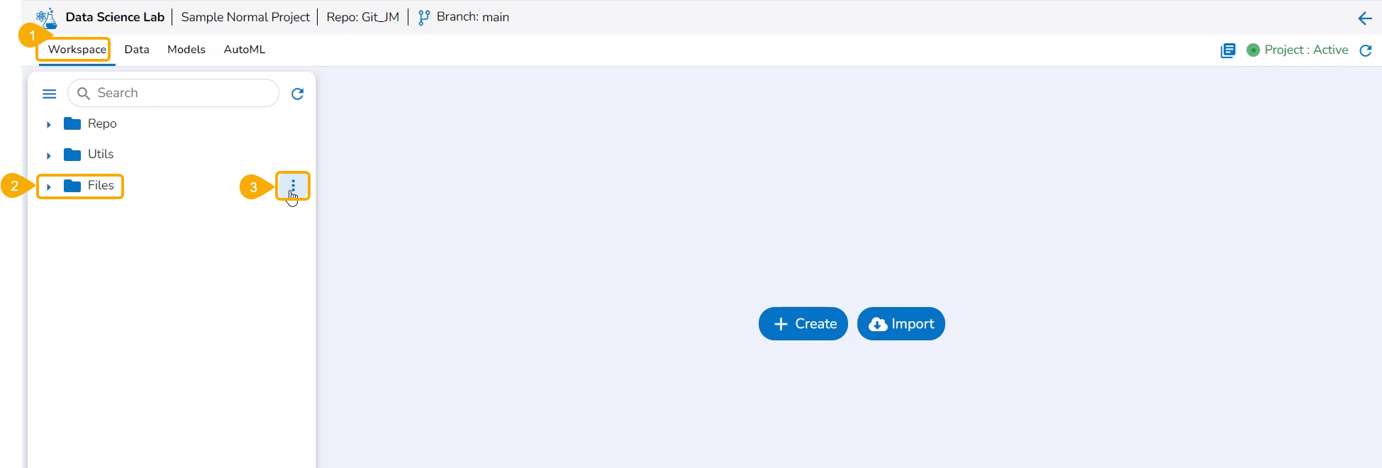
Navigate to the Workspace tab of a normal Data Science project.
Select the File folder that is created by default.
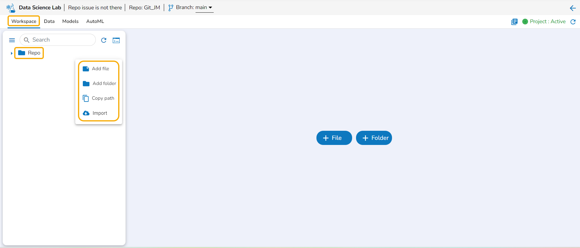
Click the Ellipsis icon for the File folder.
The credited attributive will be listed in the context menu.
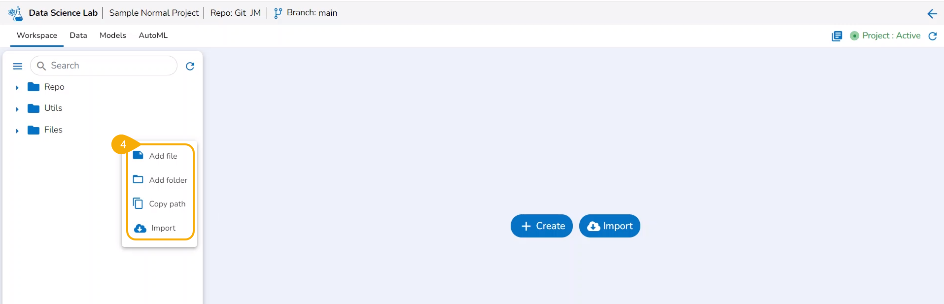
File Folder Attributives
Add File
Check out the illustration on adding a file to the File folder of a normal Data Science Project.
Add Folder
Check out the illustration on adding a folder to the File folder of a normal Data Science Project.
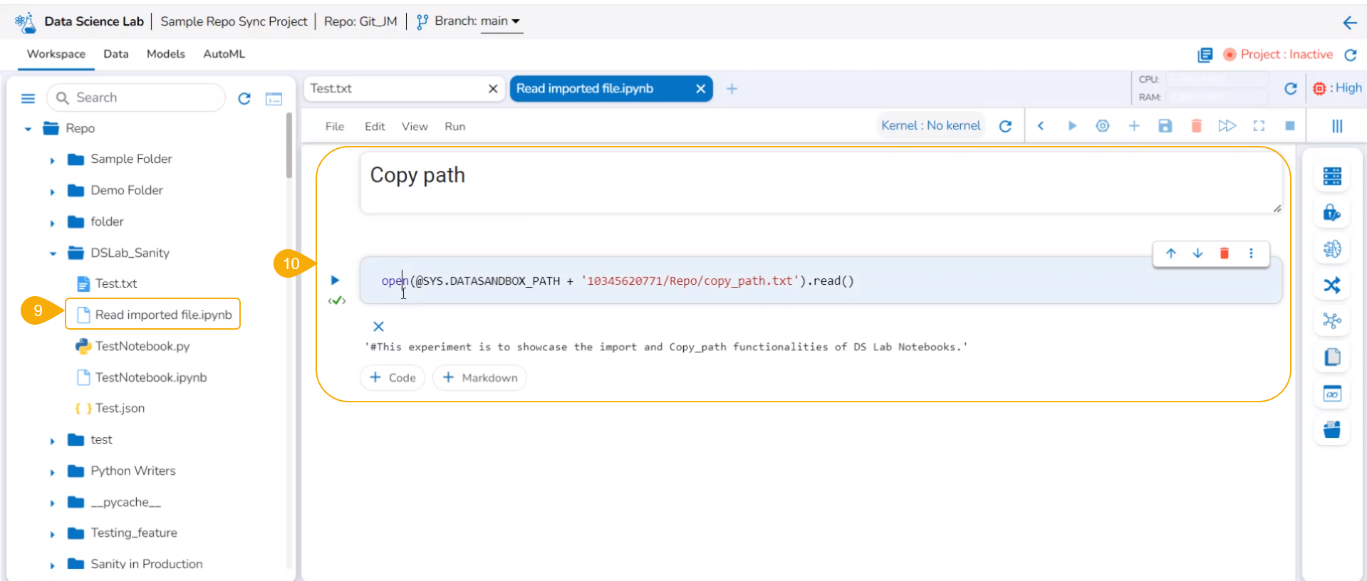
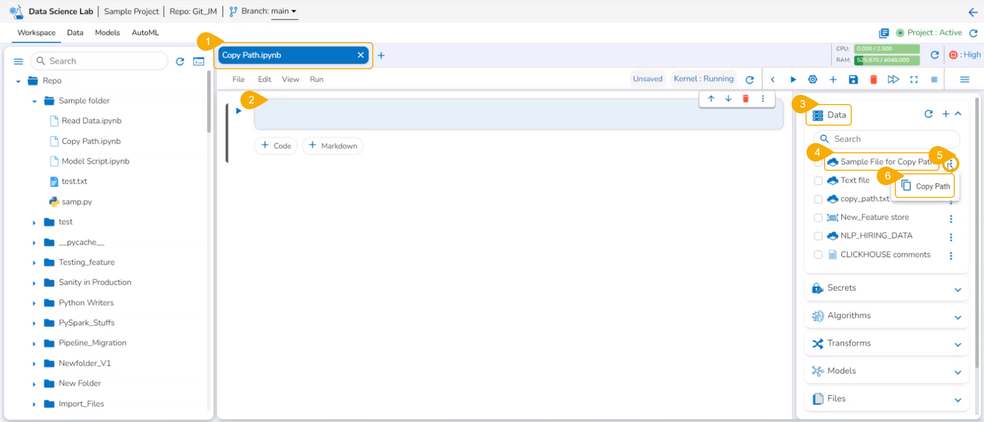
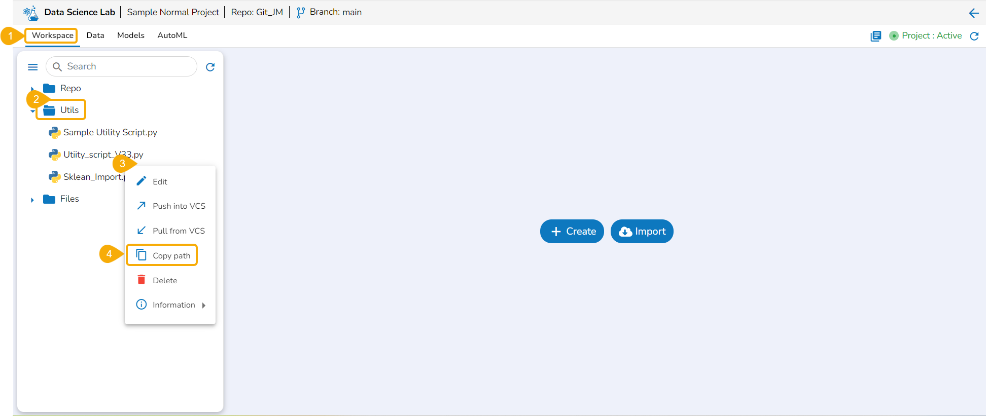
Copy path
Check out the illustration on using the Copy path functionality inside the File folder of a normal Data Science Project.
Import
Check out the illustration on importing a file to the File folder of a normal Data Science Project.
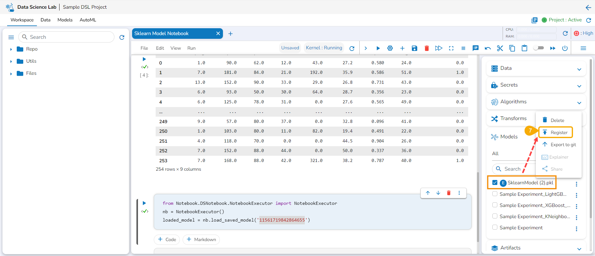
Check out the walk-through to Register a Data Science model to the Data Pipeline (from the Model tab).
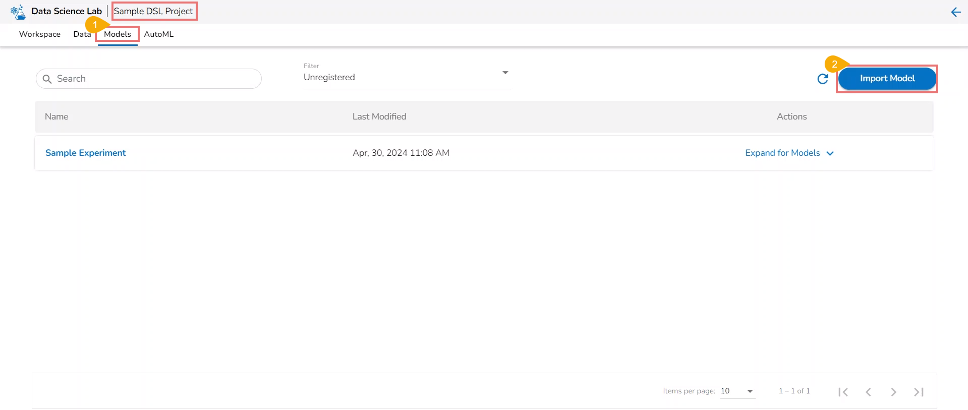
The user can export a saved DSL model to the Data Pipeline module from the Modelstab.
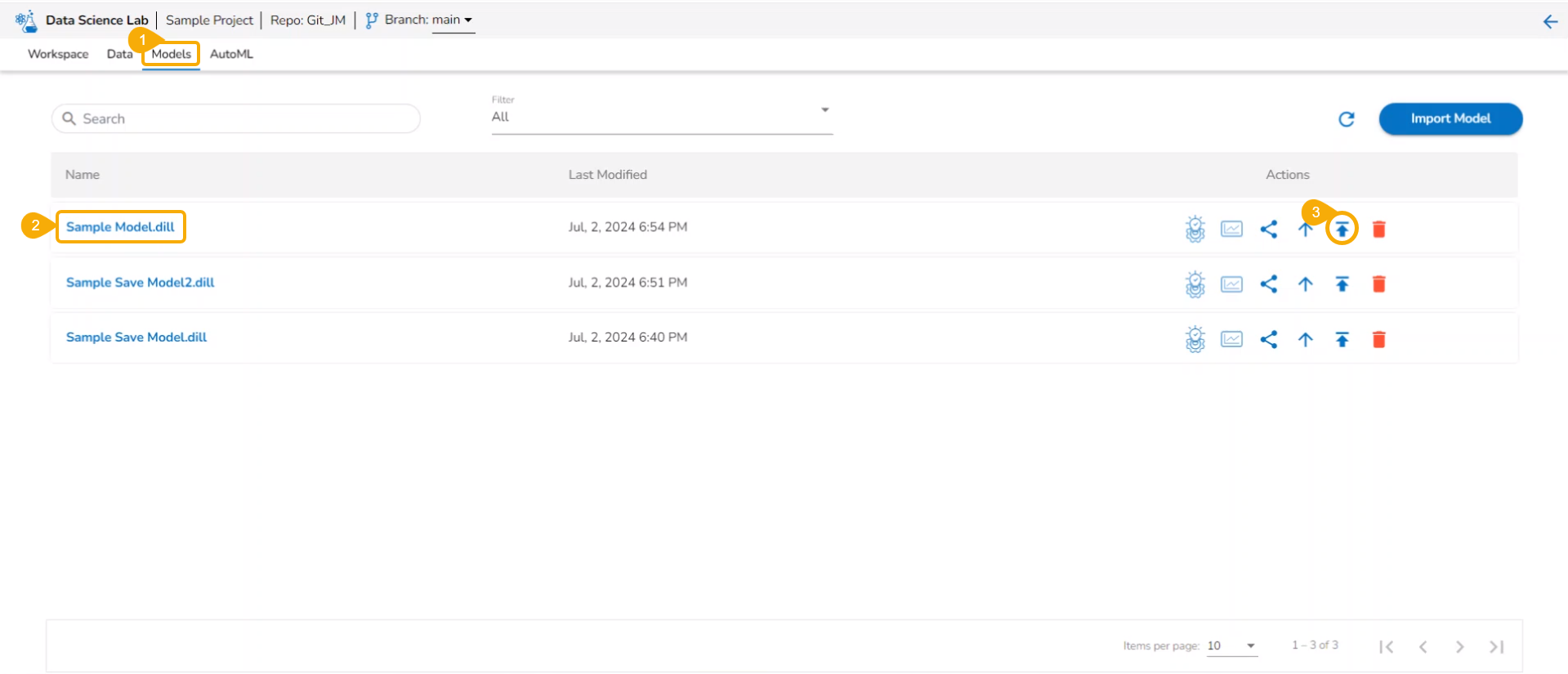
Navigate to the Models tab.
Select a model (unregistered model) from the list.
Click the Register icon for the model.
Register option for a model on the Model tab
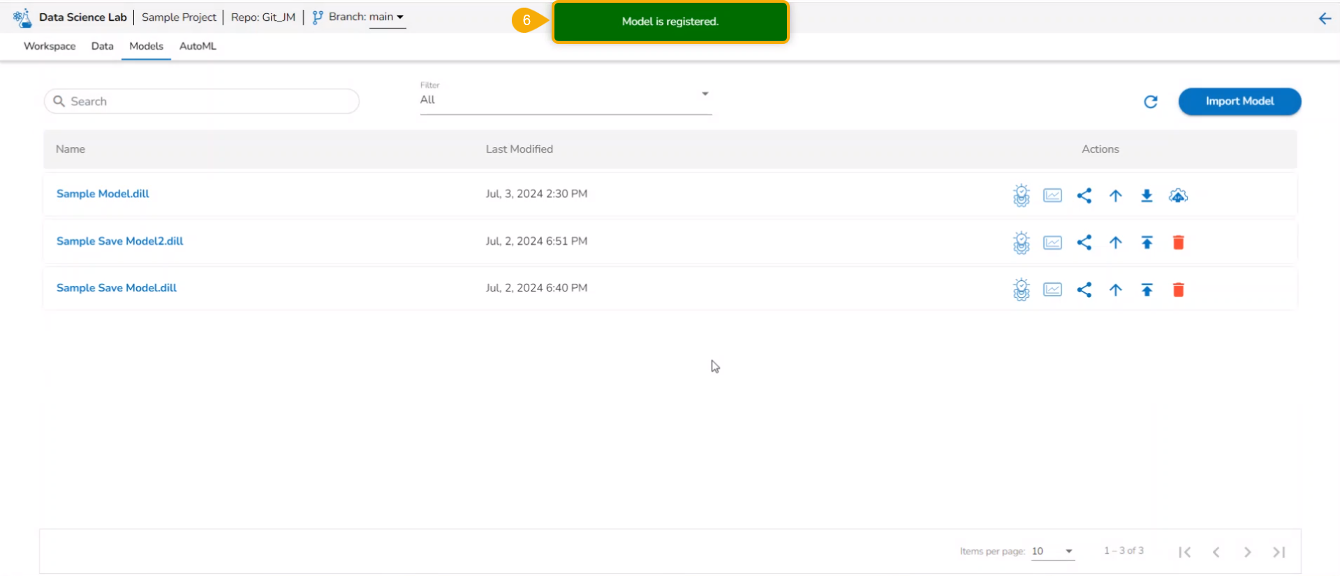
The Register dialog box appears to confirm the action.
Click the Yes option.
A notification message appears to inform the same.
Please Note: The registered model gets published to the Data Pipeline (it is moved to the Registered list of the models).
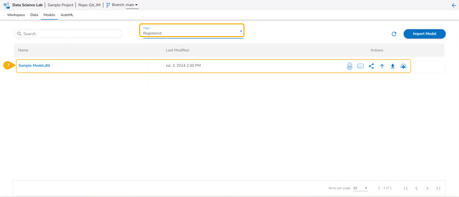
The model gets listed under the Registered model list.
Please Note:
TheRegister option is also available under the Models section inside a Data Science Notebook.
The Registered Models can be accessed within the DS Lab Model Runner component of the Data Pipeline module.
Models
tab.
Select an unregistered model filter option.
Select a model from the displayed list.
Click the Delete icon.
A confirmation message appears.
Click the Yes option.
A notification message appears.
The selected model gets deleted.
Please Note: The Delete icon appears only for the unregistered models. The registered models will not get the Delete icon.
The Save as Notebook dialog box opens.
Click the Yes option.
The current Notebook gets closed and a notification message appears to assure the user that all the recent changes are saved in it.
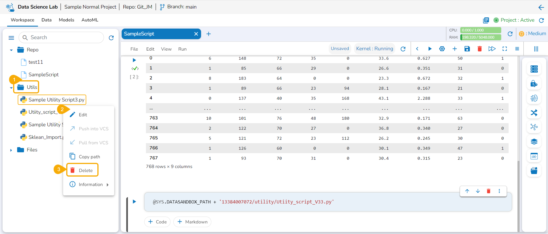
Click on the ellipsis icon provided for the selected Notebook.
A Context menu appears. Click the Delete option from the Context menu.
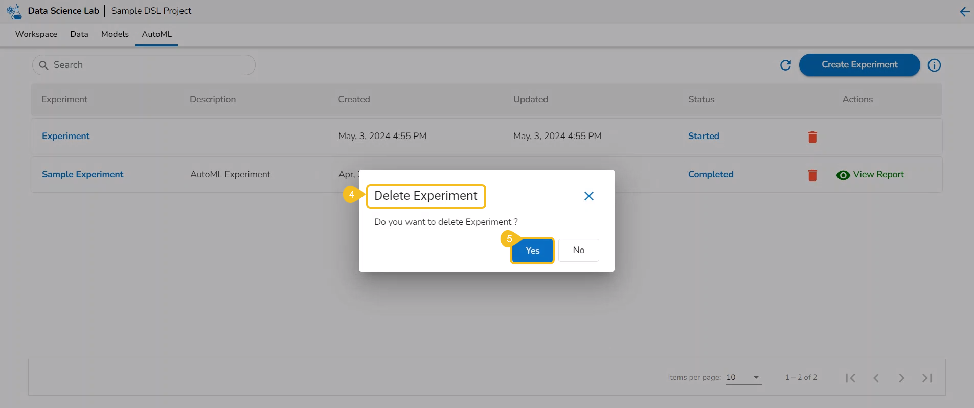
The Delete Notebook dialog box appears for the deletion confirmation.
Click the Yes option.
A notification appears to ensure the successful removal of the selected Notebook. The concerned Notebook gets removed from the Repo folder.
Project Container is inactive
Project container is initializing
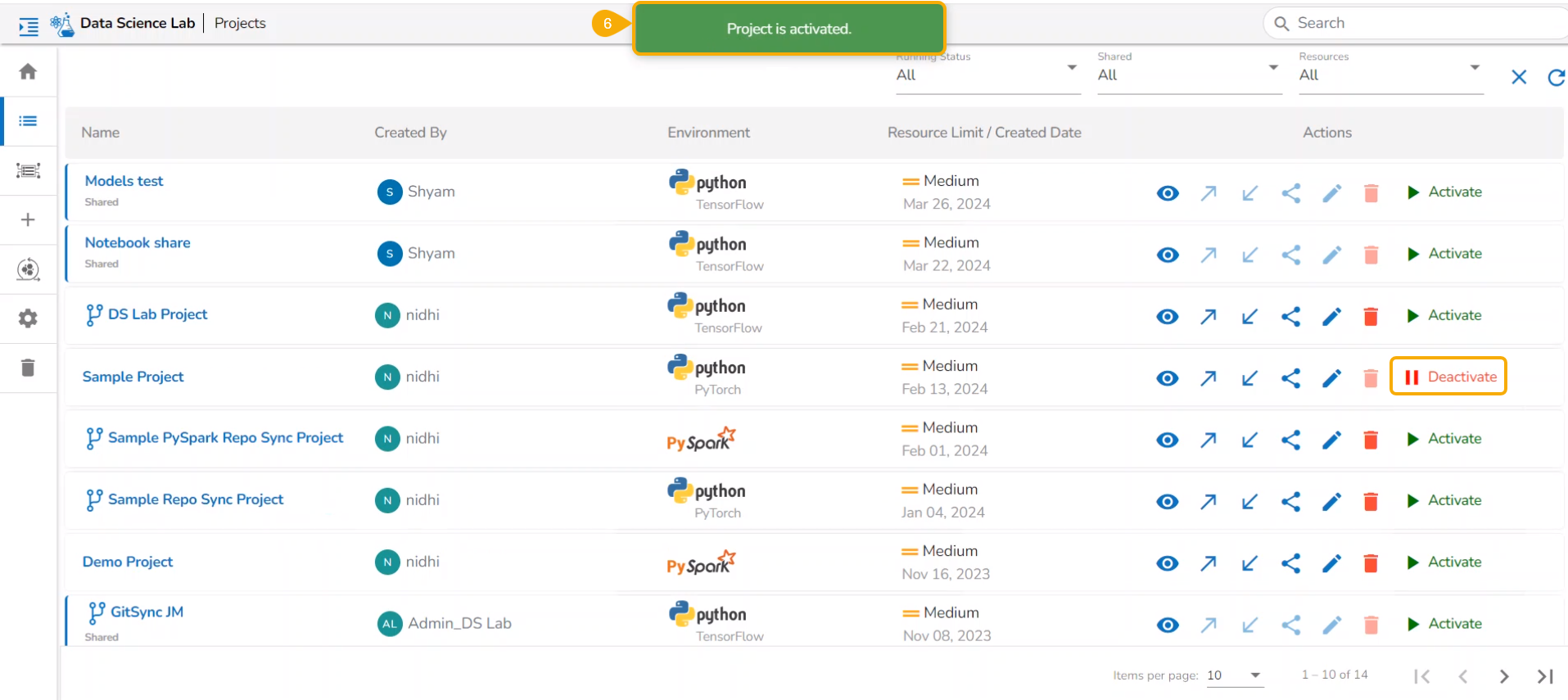
Project container is active
Trash
The Trash page lists all the deleted Projects and Feature Stores.
The Trash page will display the deleted Projects and Feature Stores accessible for the logged in user. The user gets options to Restore them or Delete them permanently from this page.
Restoring a Project
Check out the given workflow to restore a project.
Navigate to the Data Science Lab Homepage.
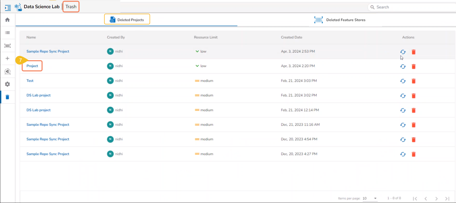
Click the Trash icon provided in the left-side menu panel.
The Trash page opens displaying two tabs:
Deleted Projects
Deleted Feature Stores
Select a Project from the displayed list of the Deleted Projects.
Click the Restore icon.
A dialog message appears to confirm the selected action.
Click Yes to confirm the action.
A notification message appears.
The concerned project gets restored to the Projects list.
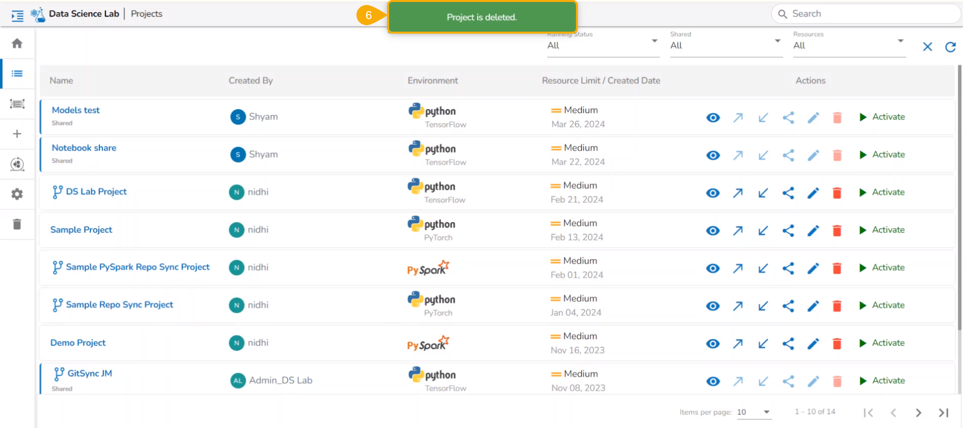
Deleting a Project Permanently
Check out the given workflow to delete a project permanently.
Navigate to the Data Science Lab Homepage.
Click the Trash icon provided in the left-side menu panel.
The Trash page opens displaying two tabs:
Deleted Projects
Deleted Feature Stores
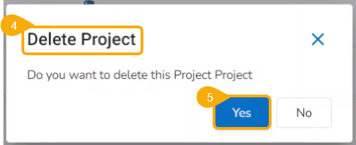
Select a Project from the displayed list.
Click the Delete icon.
A dialog message appears to confirm the selected action.
Click Yes to confirm the action.
A notification message appears, and the selected Project gets removed permanently from the Data Science Lab module.
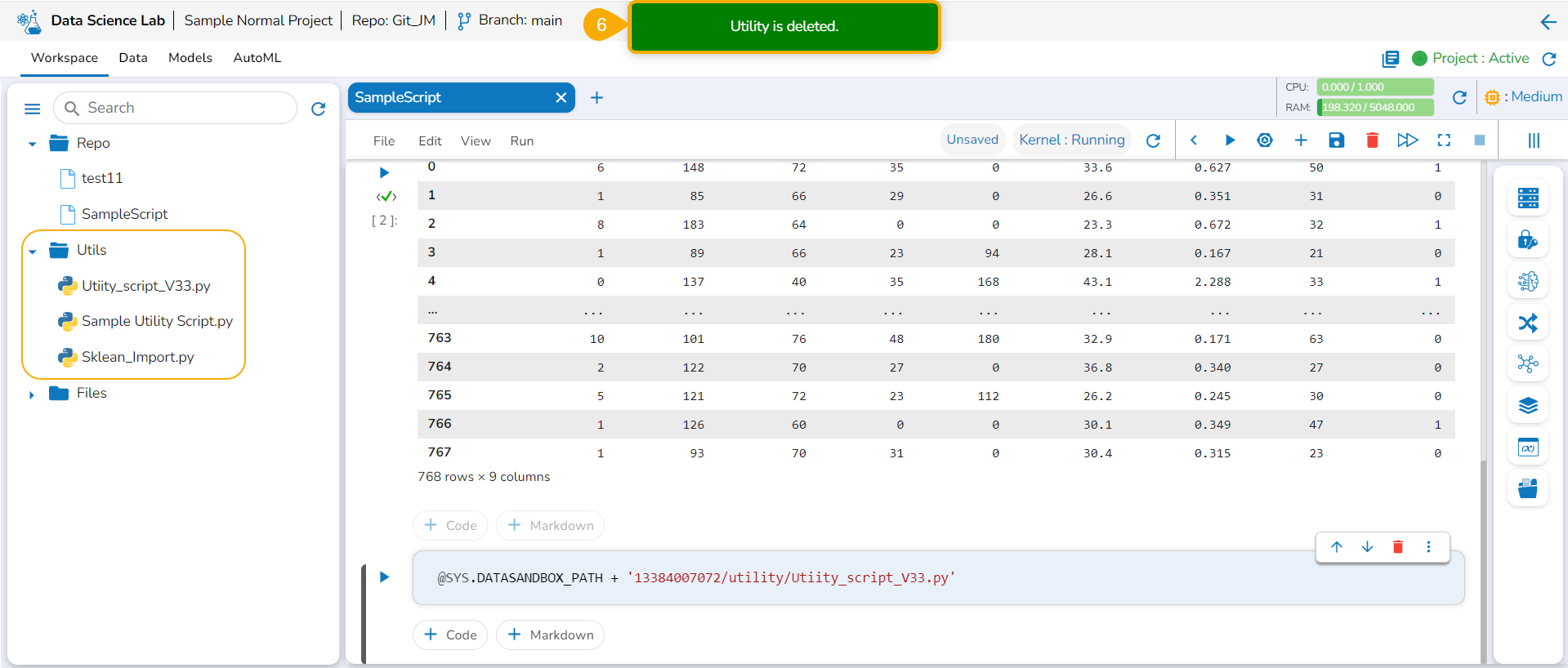
Utils Folder Attributes
This section explains the attributive action provided for the Utils folder.
Accessing Utilis Folder
The Utilis folder allows the users to import the utility files from their systems and Git repository.
Please Note: The Utils folder will be added by default to only normal Data Science Lab projects.
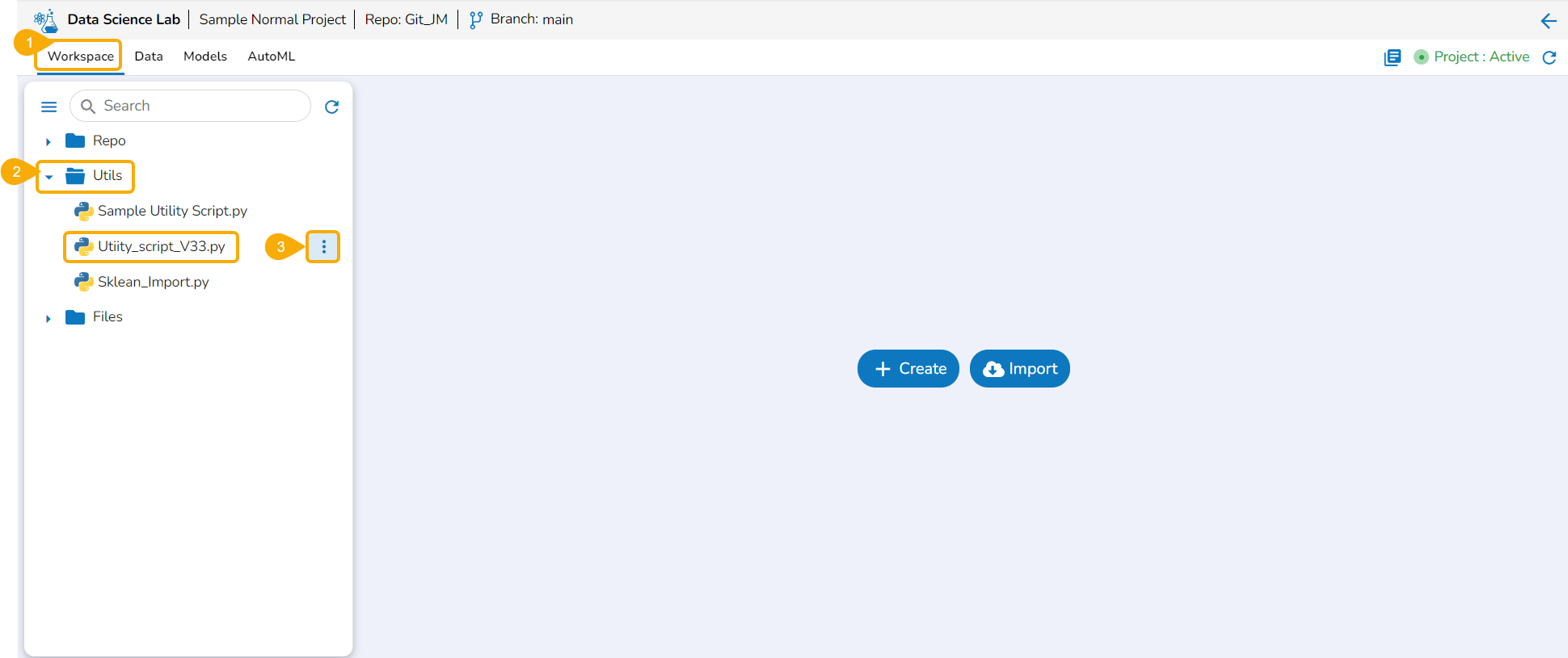
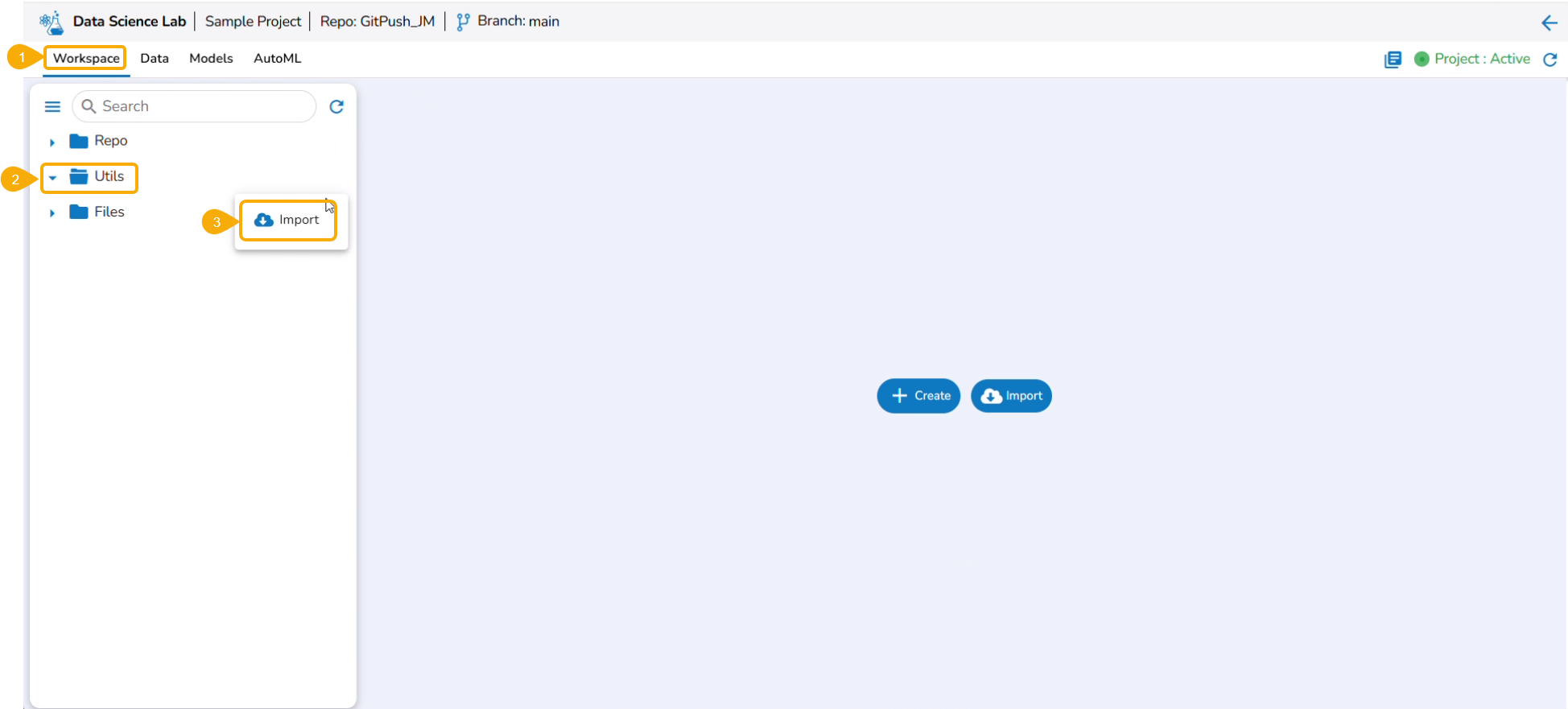
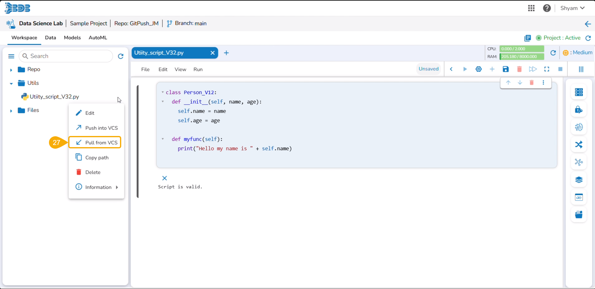
Navigate to the Workspace tab.
Select the Utils folder.
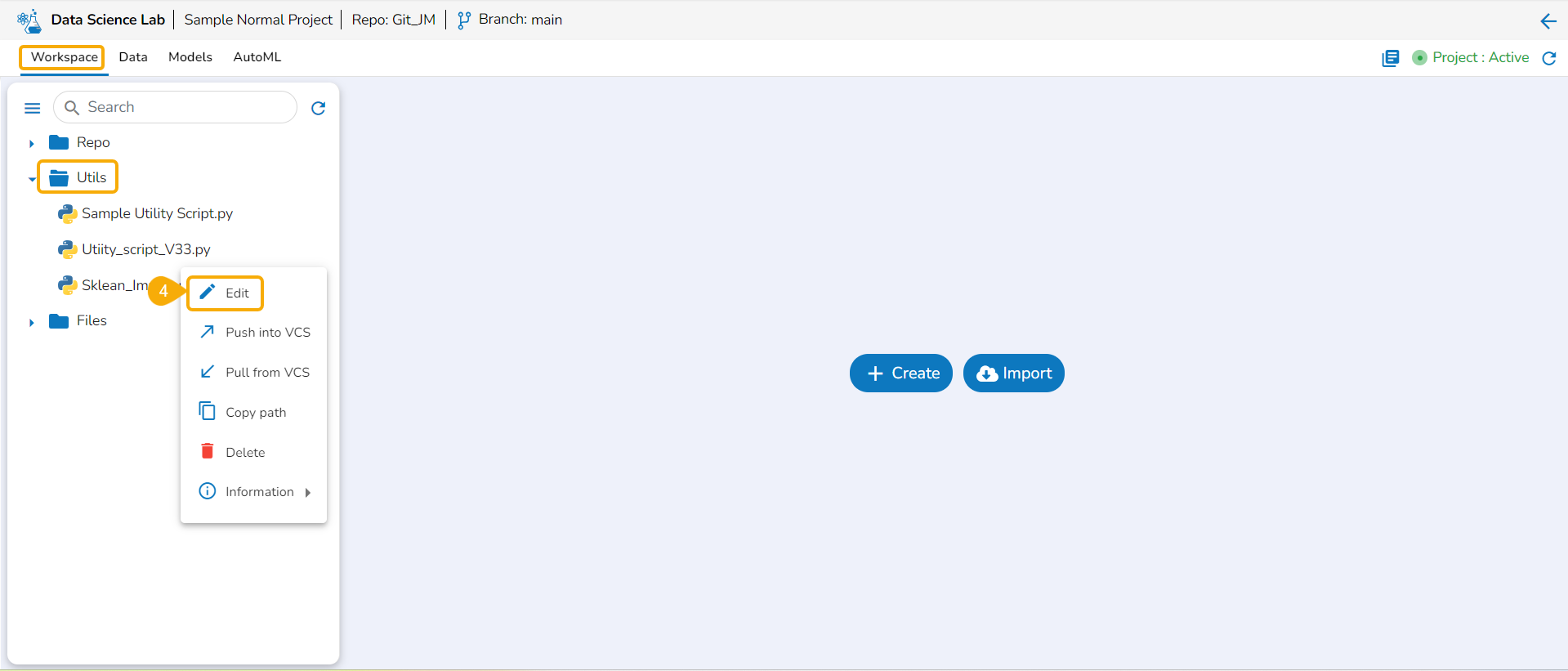
Click the ellipsis icon to open the context menu.
Click the Import option that appears in the context menu.
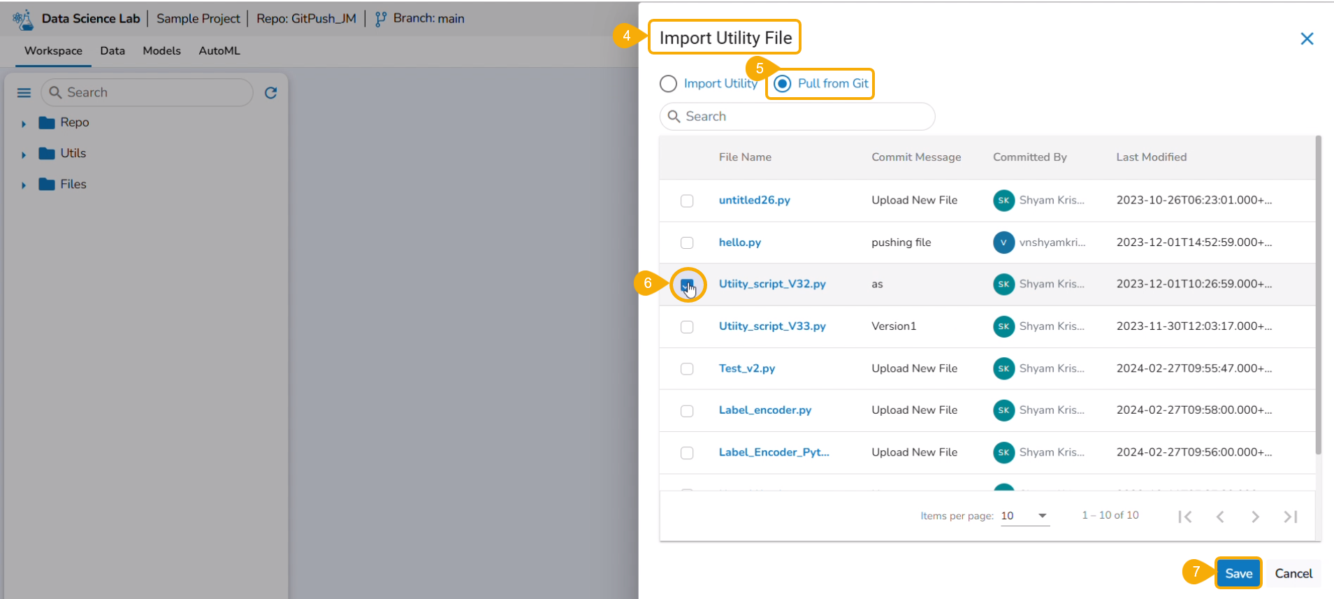
The Import Utility File window opens.
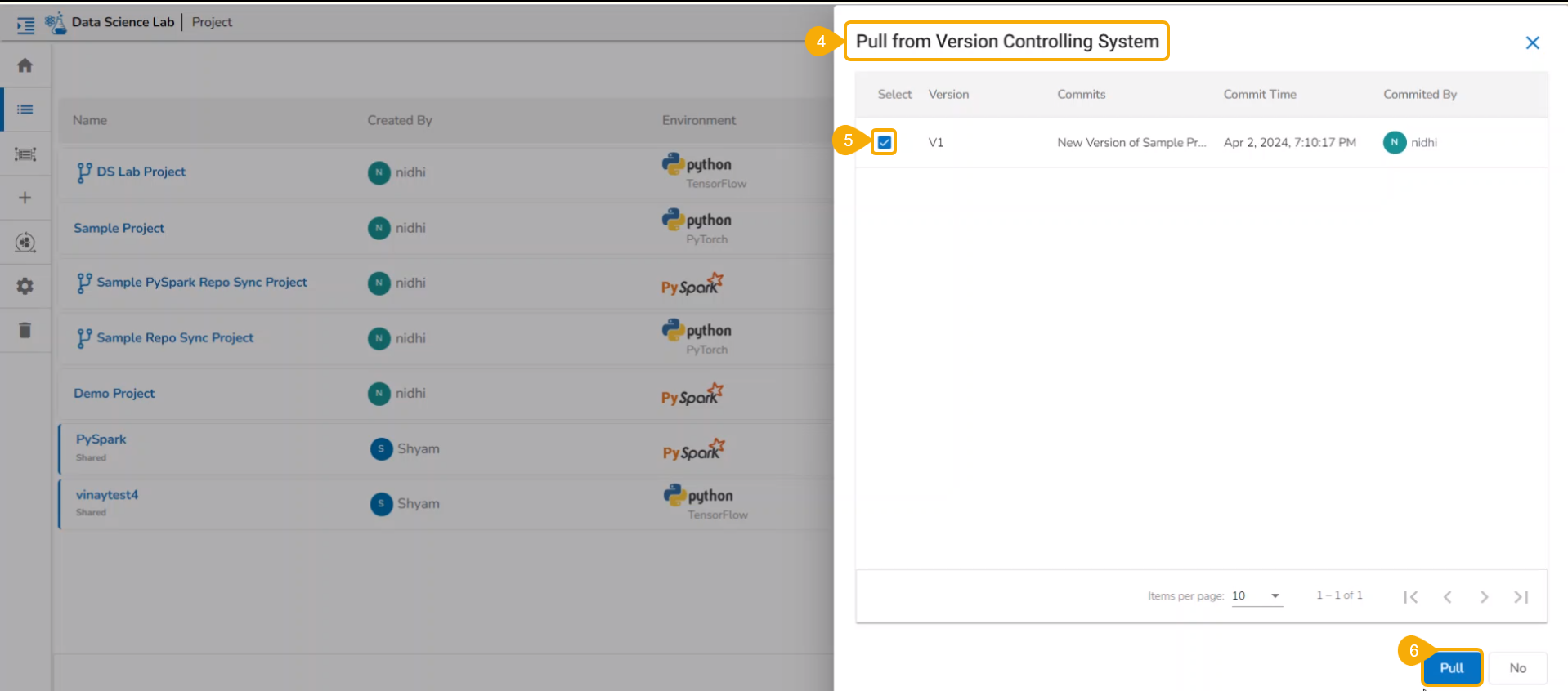
The user can import a utility file using either of the options: Import Utility or Pull from Git.
Importing a Utility File
Check out the walk-through video to understand the Import Utility functionality.
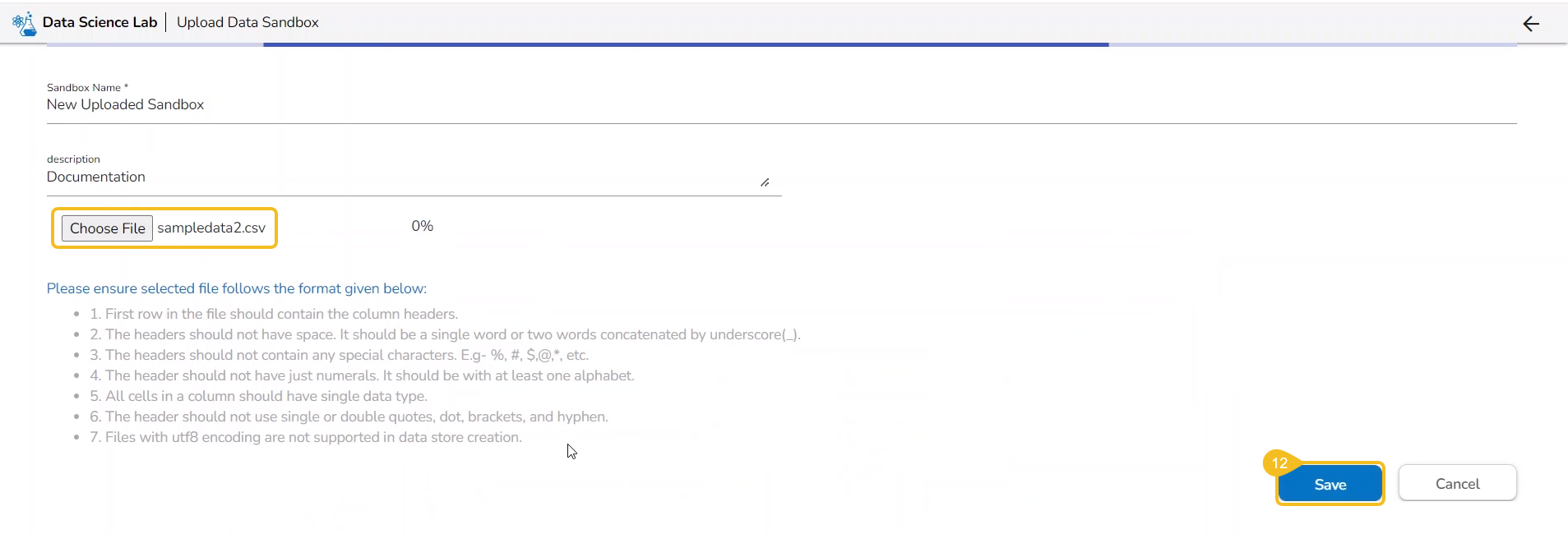
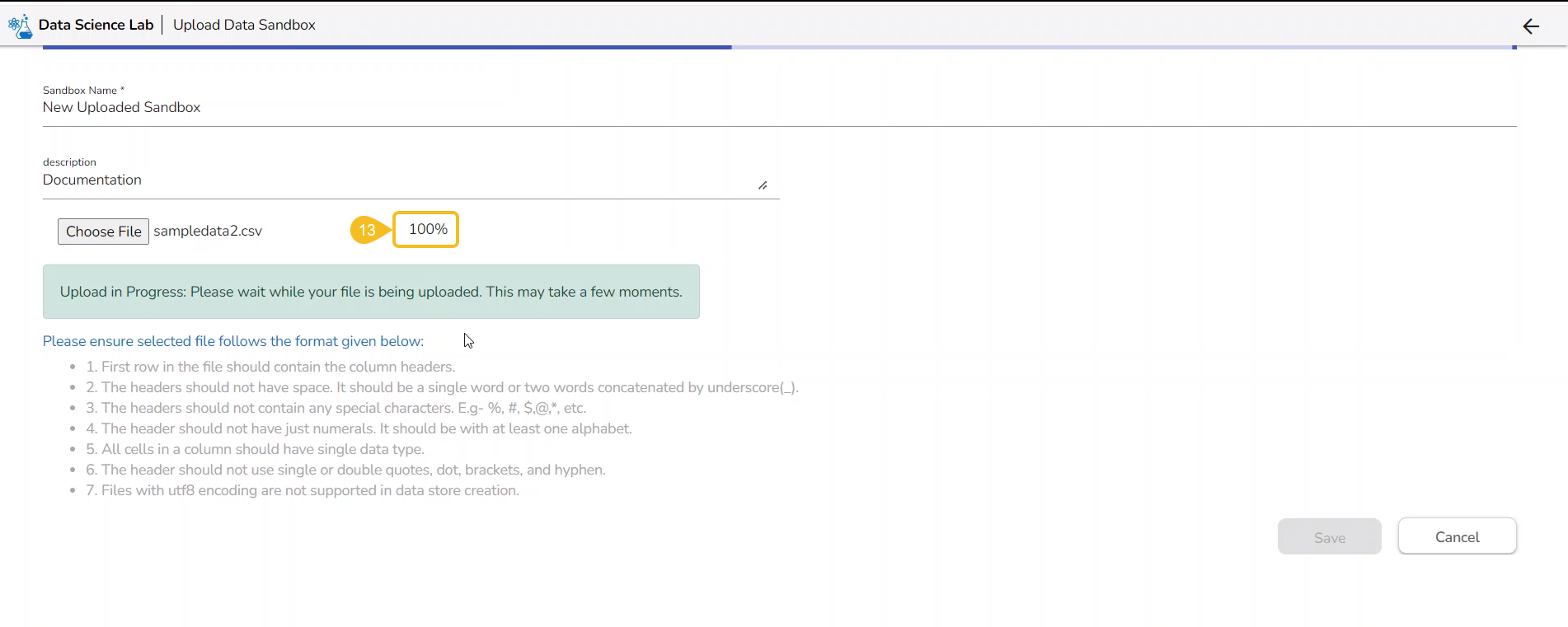
Navigate to the Import Utility File window.
Select the Import Utility option by using the checkbox.
Describe the Utility script using the Utility Description space.
Search and upload a utility file from the system.
The uploaded utility file title appears next to the Choose File option.
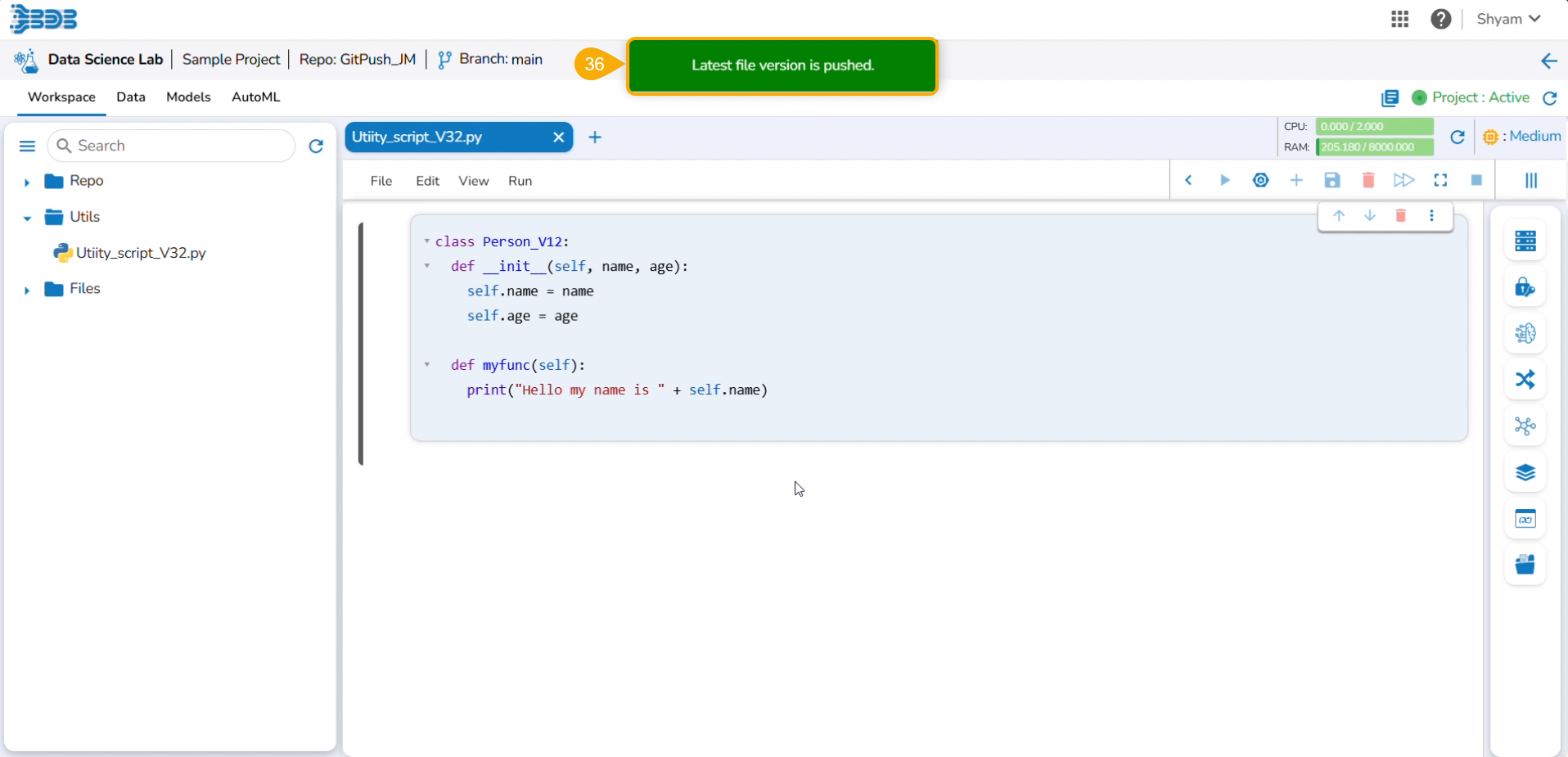
Click the Save option.
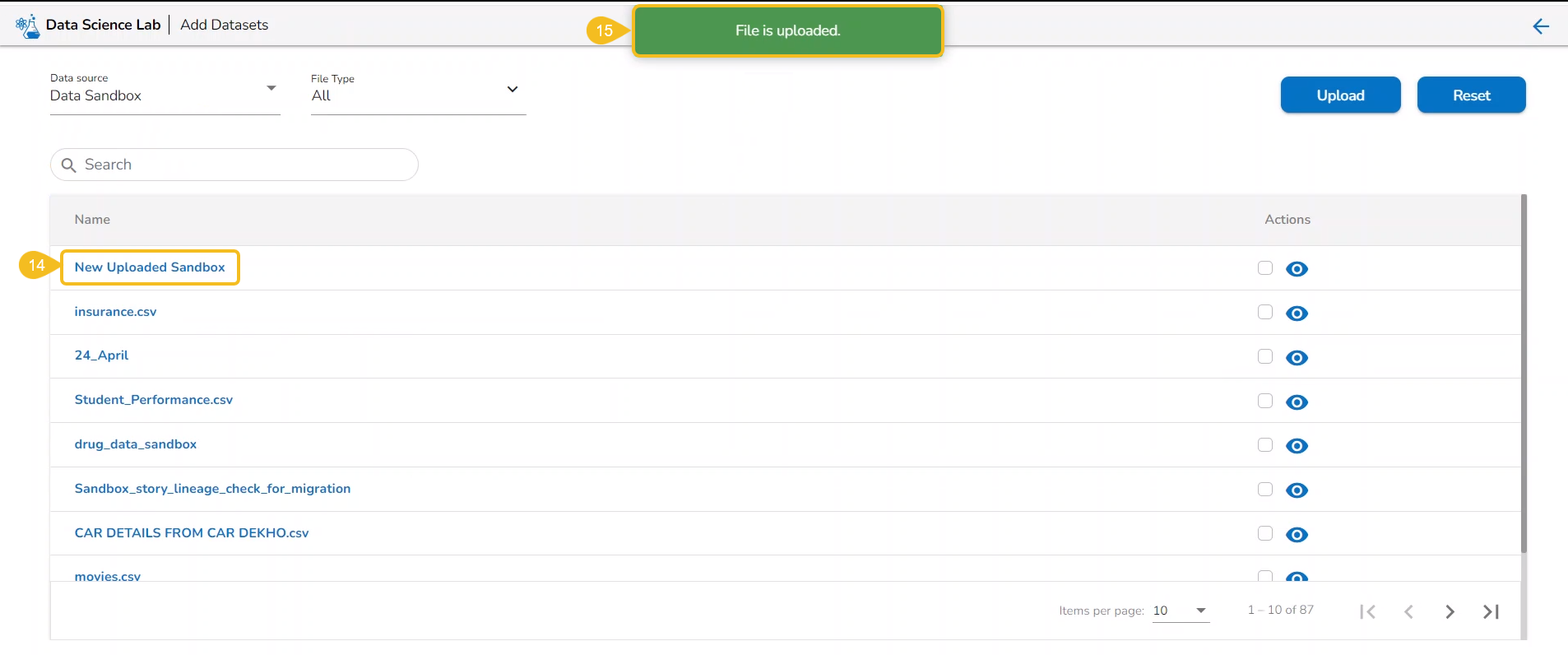
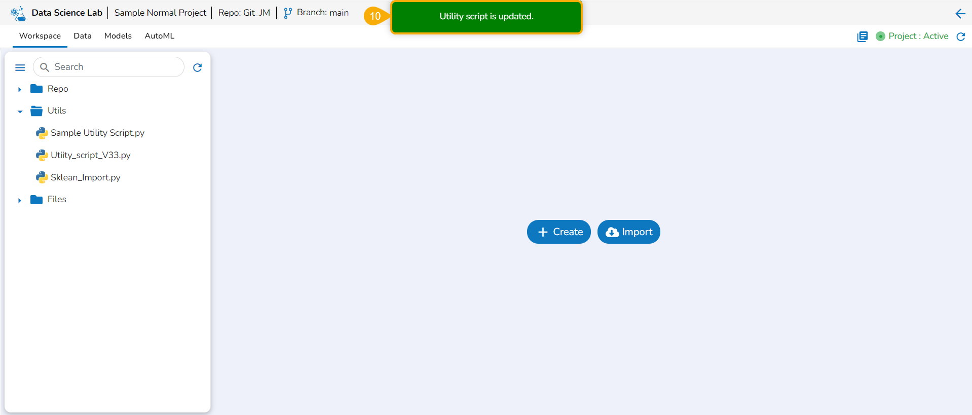
The imported utility file will display completed 100% when imported completely.
A notification also ensures that the file has been imported.
Open the Utils folder provided under the Workspace tab.
The imported utility file appears under the Utils folder.
Expanding and Collapsing Markdown Cell
The user can expand and collapse the multiple Markdown cells based on their levels in a DS Notebook. The user can create a hierarchy of three levels using the Heading option in a Markdown cell.
Please Note:
The related code cells under one Markdown will fall into the same level as the Markdown.
The maximum three levels of hierarchy can be inserted for a Markdown cell using the Heading option.
Check out the following illustration on how to set the expand and collapse functionality in Markdown cells.
Navigate to a Notebook.
Access a Markdown cell.
To create a hierarchy within a Markdown cell, use the Heading button.
Check out the illustration to see the Markdown expand and collapse feature at work.
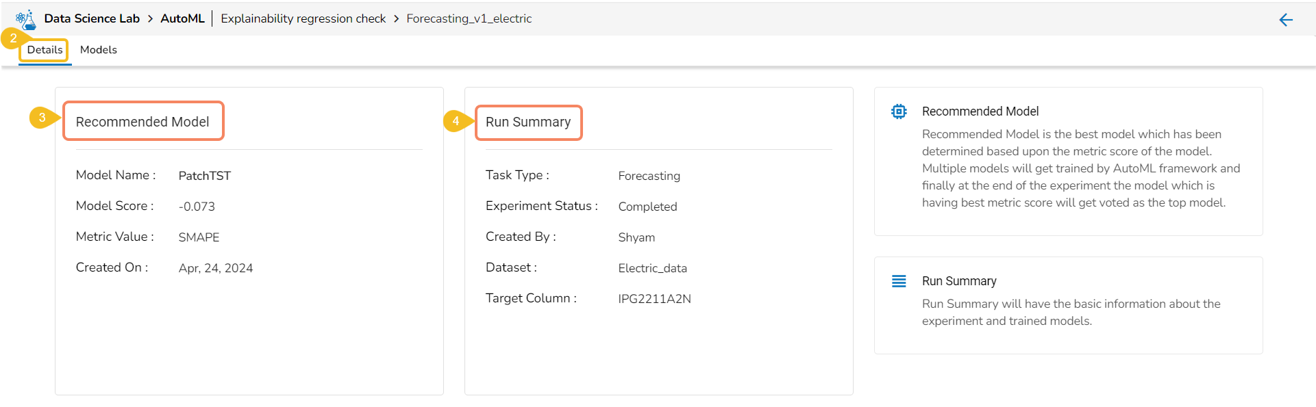
Forecasting Model Explainer
This page provides model explainer dashboards for Forecasting Models.
Check out the given walk-through to understand the Model Explainer dashboard for the Forecasting models.
The forecasting model stats get displayed through the Timeseries visualization that presents values generated over based on the selected time.
Predictions
This chart will display predicted values generated by the timeseries model over a specific time period.
Predicted Vs Actual
This chart displays a comparison of the predicted values with the actual obsereved vlaues over a specific period of time.
Residual
It depicts difference between the predicted and actual (residuals) values over a period of time.
Predicted Vs Actual Scatter Plot
A Scatter Plot chart is displayed depicting how well the predicted values align with the actual values.
Please Note:Refer the page to get an overview of the Data Science Lab module in nutshell.
Unregister a Model
To unregister a model means to remove it from the Data Pipeline environment.
Check out the illustration on unregistering a model functionality using the Models tab.
A user can unregister a registered model by using the Models tab.
Navigate to the Models tab.
Select a registered model (use the Registered filter option to access a model).
Click the Unregister icon for the same model.
The Unregister dialog box appears to confirm the action.
Click the Yes option.
A notification message appears to inform the same.
The unregistered model appears under the Unregistered filter of the Models tab.
Please Note:
The Unregister function when applied to a registered model, gets removed from the Data Pipeline module. It also disappears from the Registeredlist of the models and gets listed under the Unregistered list of models.
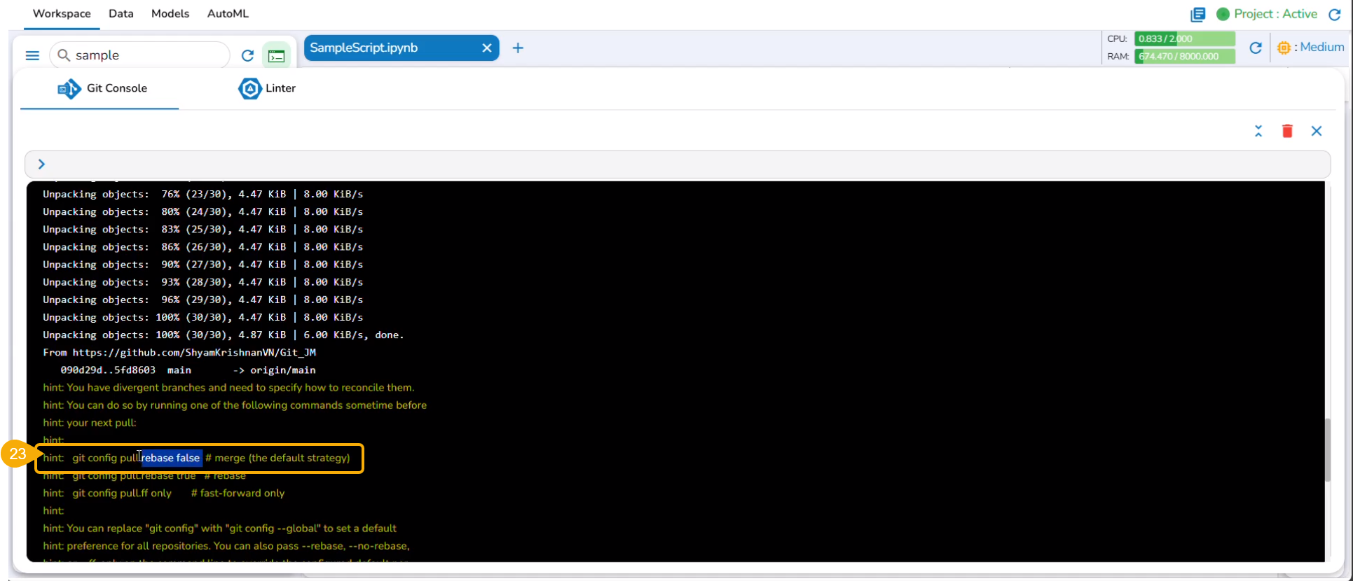
Linter
This release provides support from Linter to analyze source code and identify programming errors, bugs, and other potential issues.
The Linter functionality helps developers maintain high code quality by enforcing coding standards and best practices.
A linter helps in data science by:
Improving Code Quality: Enforces coding standards and best practices.
Detecting Errors Early: Identifies syntax errors, logical mistakes, and potential bugs before execution.
Enhancing Maintainability: Catches issues like unused variables, making code easier to maintain.
Facilitating Collaboration: Ensures consistent coding conventions across team members.
Optimizing Performance: Highlights inefficient code patterns for better performance in data processing and analysis.
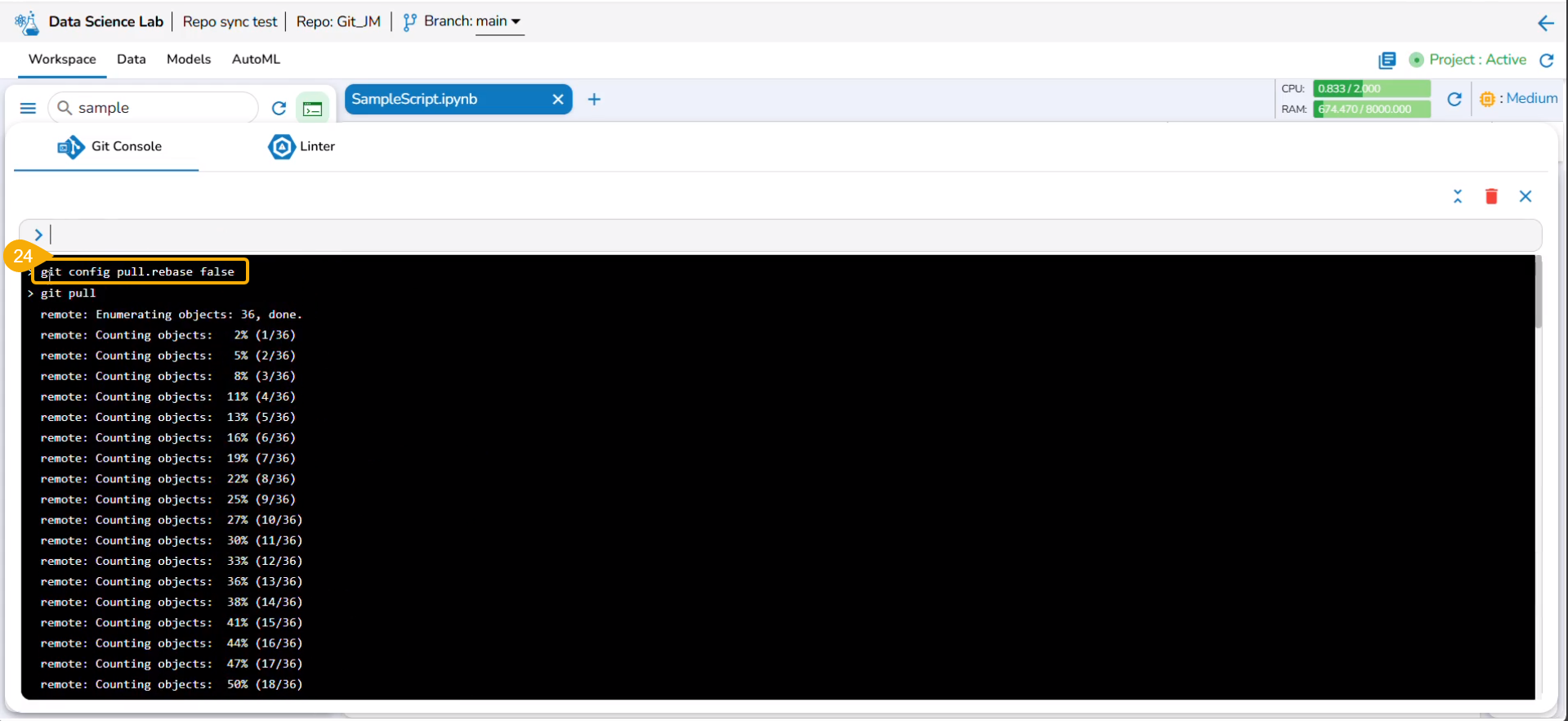
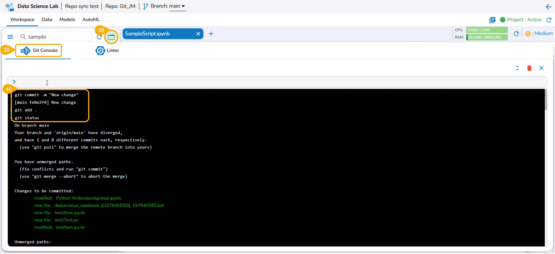
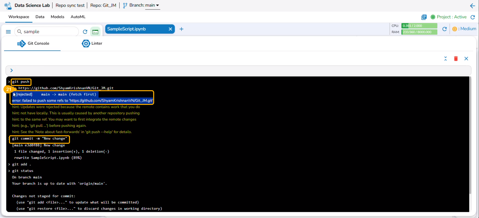
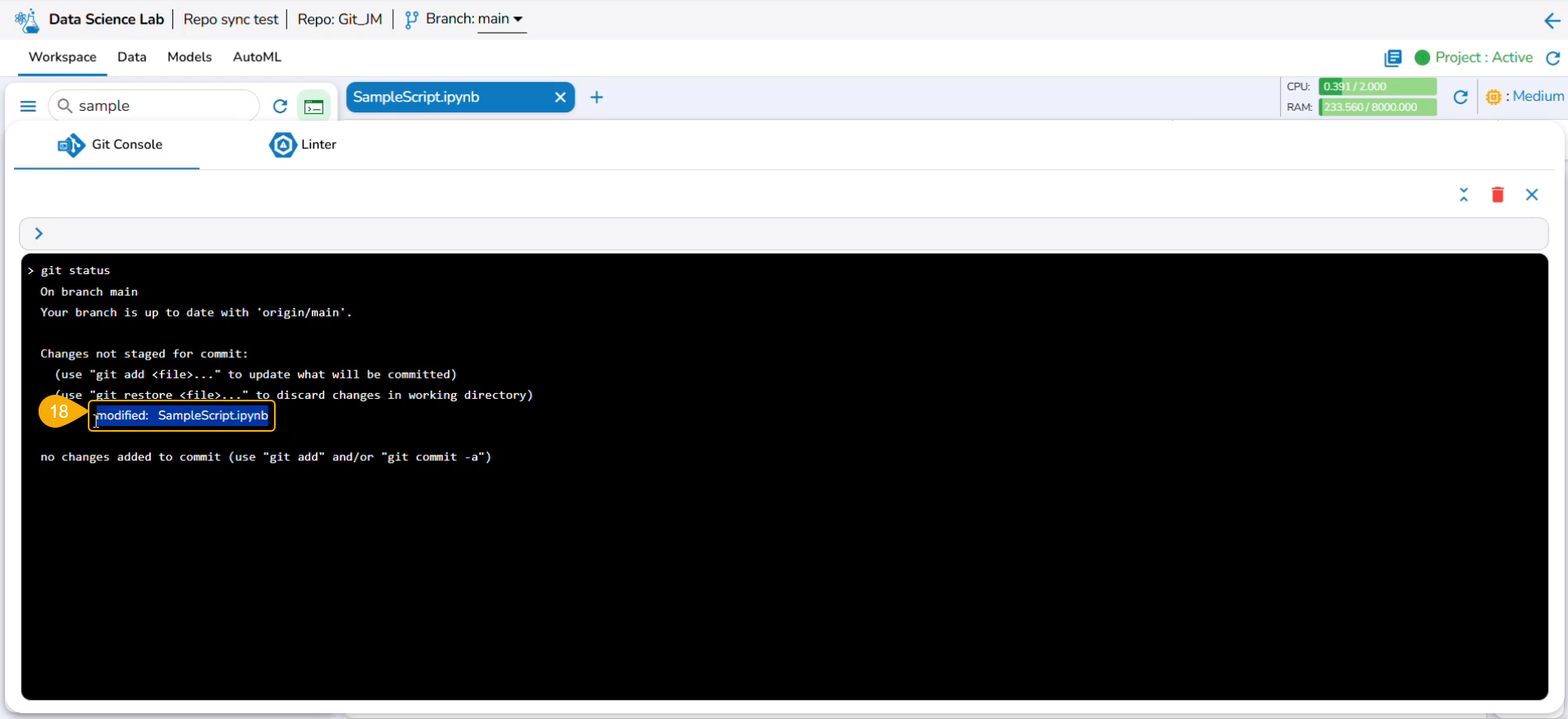
Please Note: The Linter functionality is available for normal and Repo Sync projects. The Repo Sync Projects display the Git Console as well in the drawer that appears while using the Linter functionality.
Check out the illustration on how Linter functionality works.
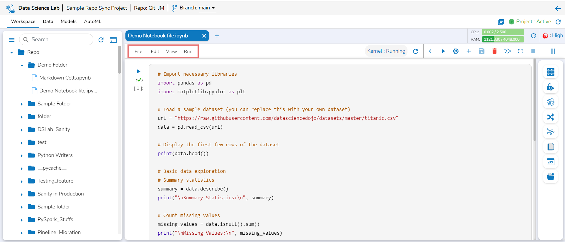
Notebook Operations
This section aims at describing the various operations for a Data Science Notebook.
Please Note: The Notebook Operations may differ based on the selection of the project environments. A notebook created under the PySpark environment only supports Data, Secrets, Variable Explorer, and Writers operations.
A Data Science Notebook created under the PyTorch or TensorFlow environment will contain the following operations:
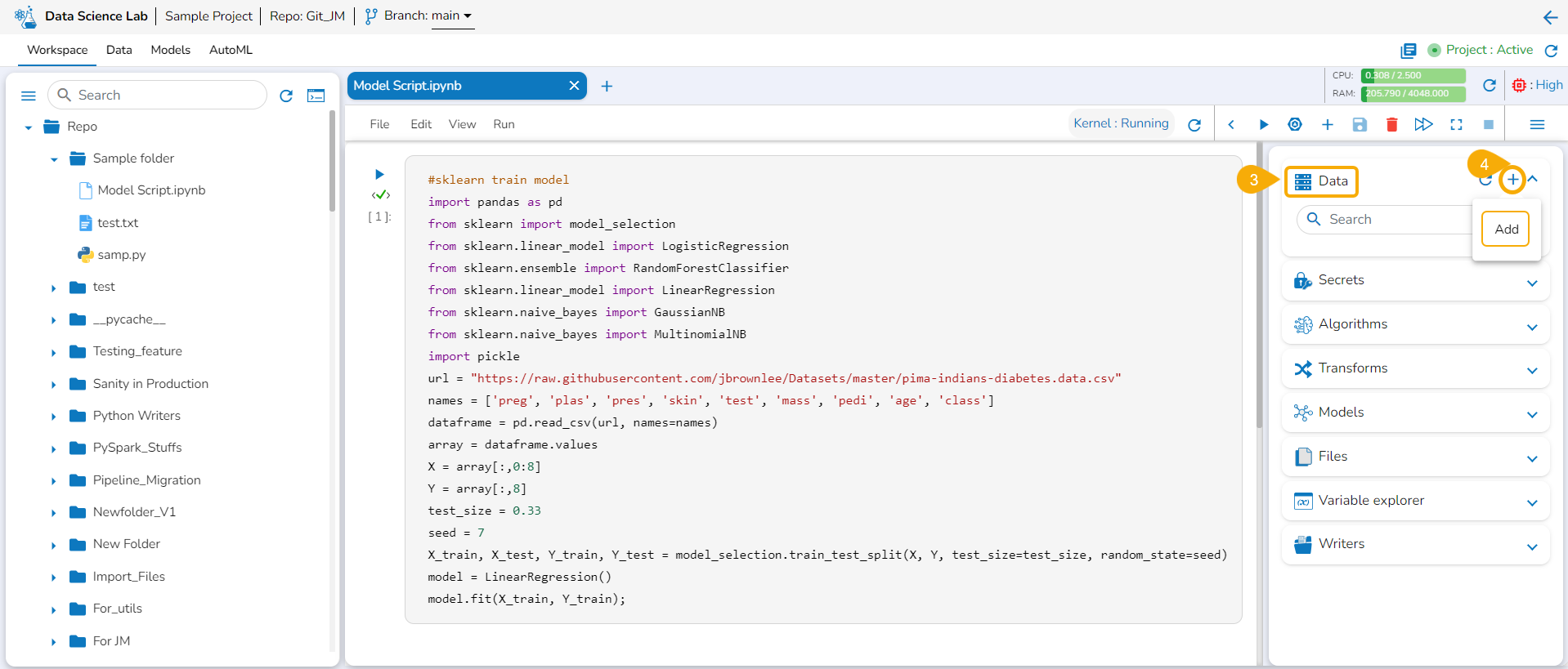
Data: Add data and get a list of all the added datasets.
Secrets: You can generate Environment Variables to save your confidential information from getting exposed.
Algorithms: You can get steps to do Algorithm Settings and Project-level access to use Algorithms inside Notebook.
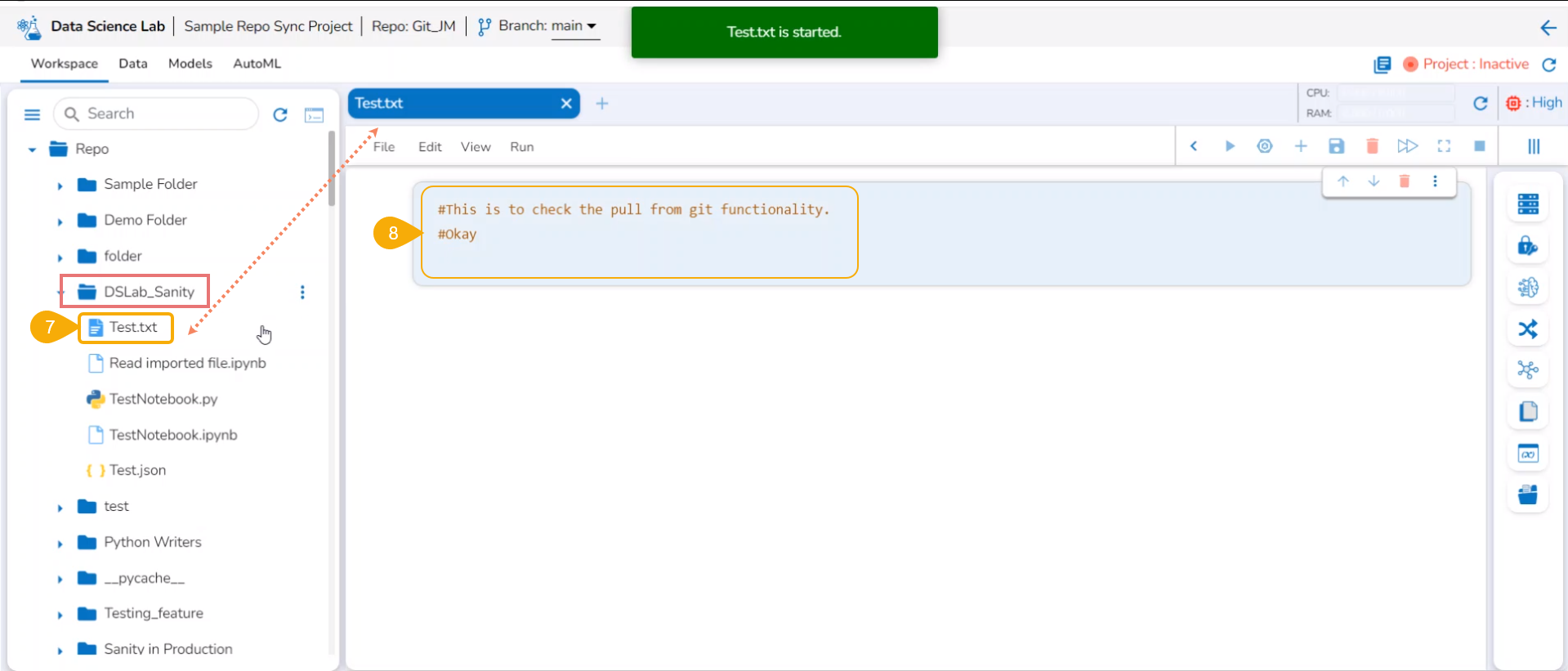
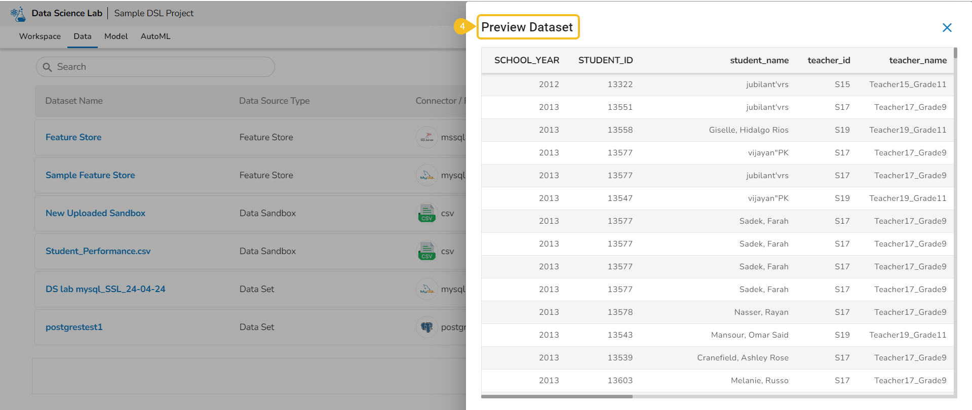
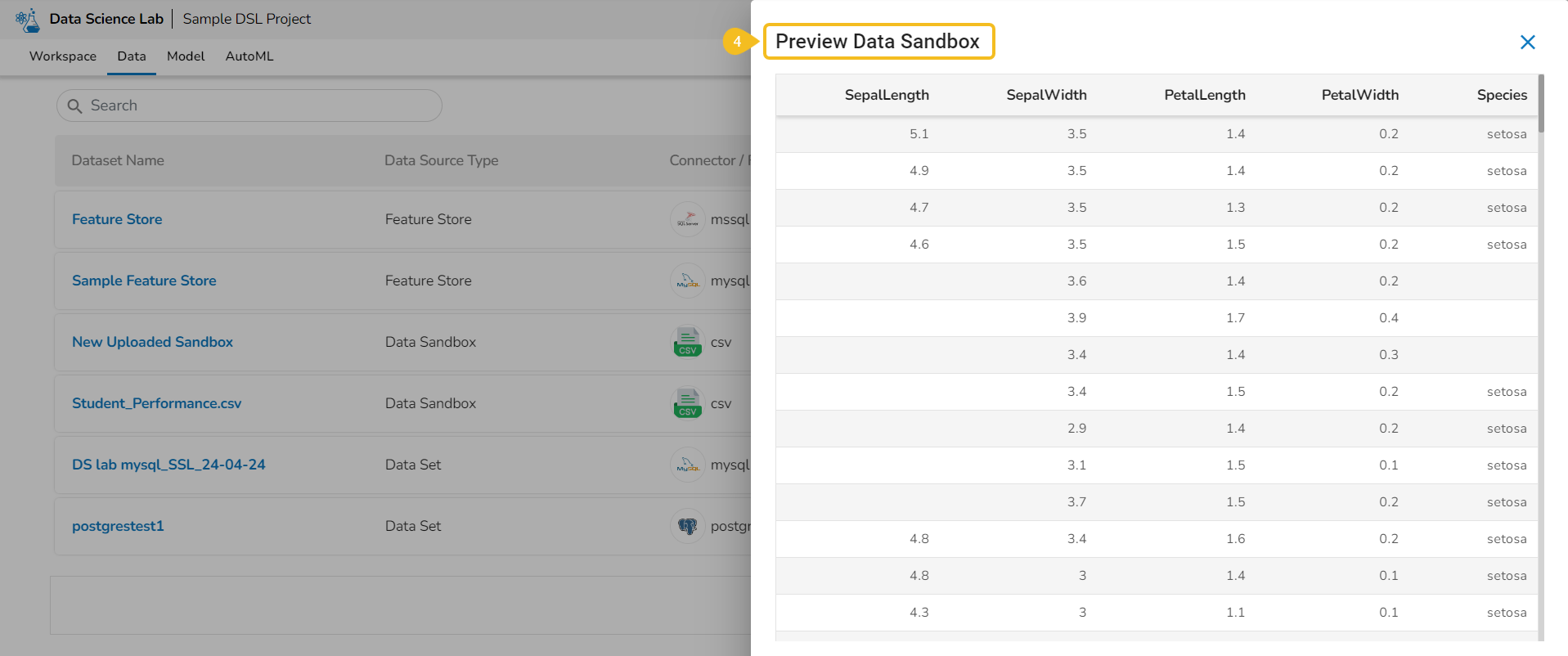
Preview File
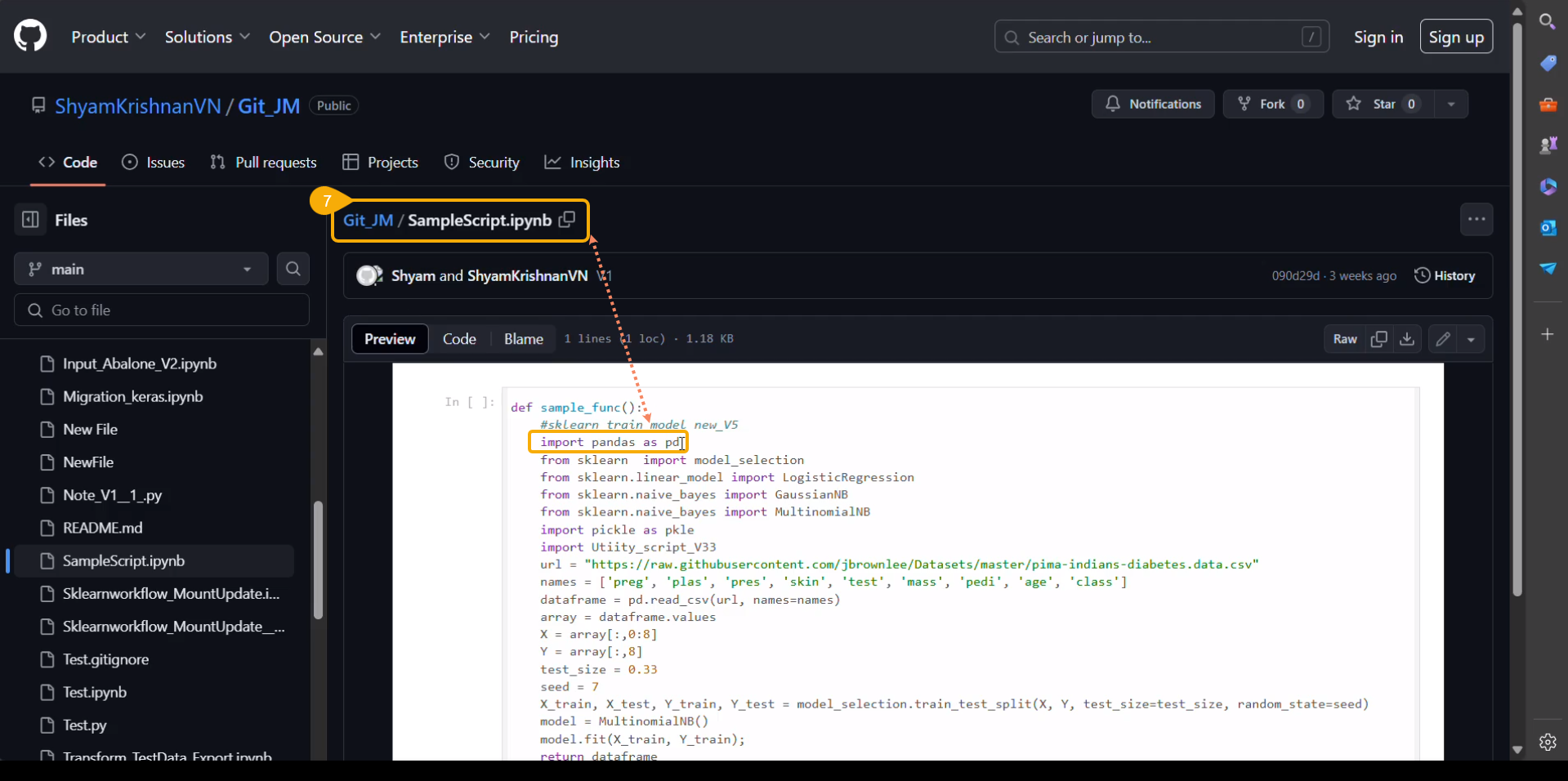
A Data Science Notebook (.ipynb files) page can be opened, and code & markdown cells can be previewed without activating the respective project.
Check out the illustration to understand the preview file content inside a project.
Please Note: A Repo Sync project contains all the files under the Repo folder. A Normal project contains only Data Science Notebook(.ipynb) files under the Repo folder.
The user can preview the content saved under any file without activating the Project where it is saved.
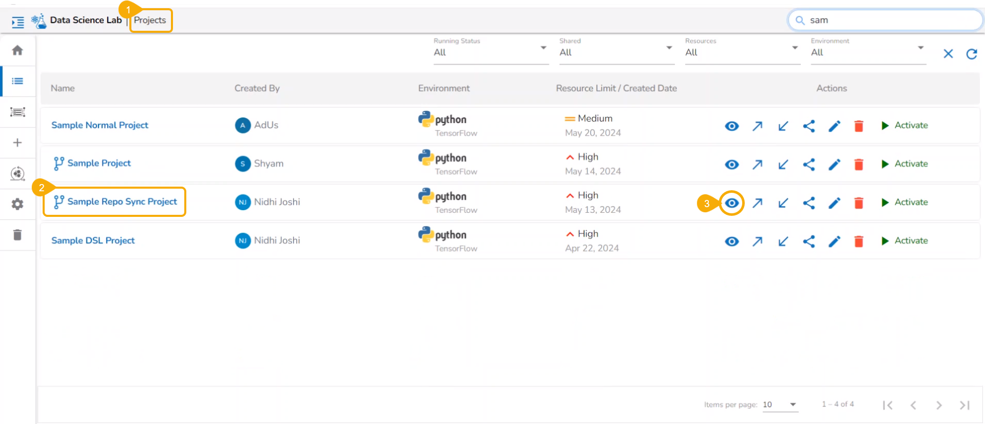
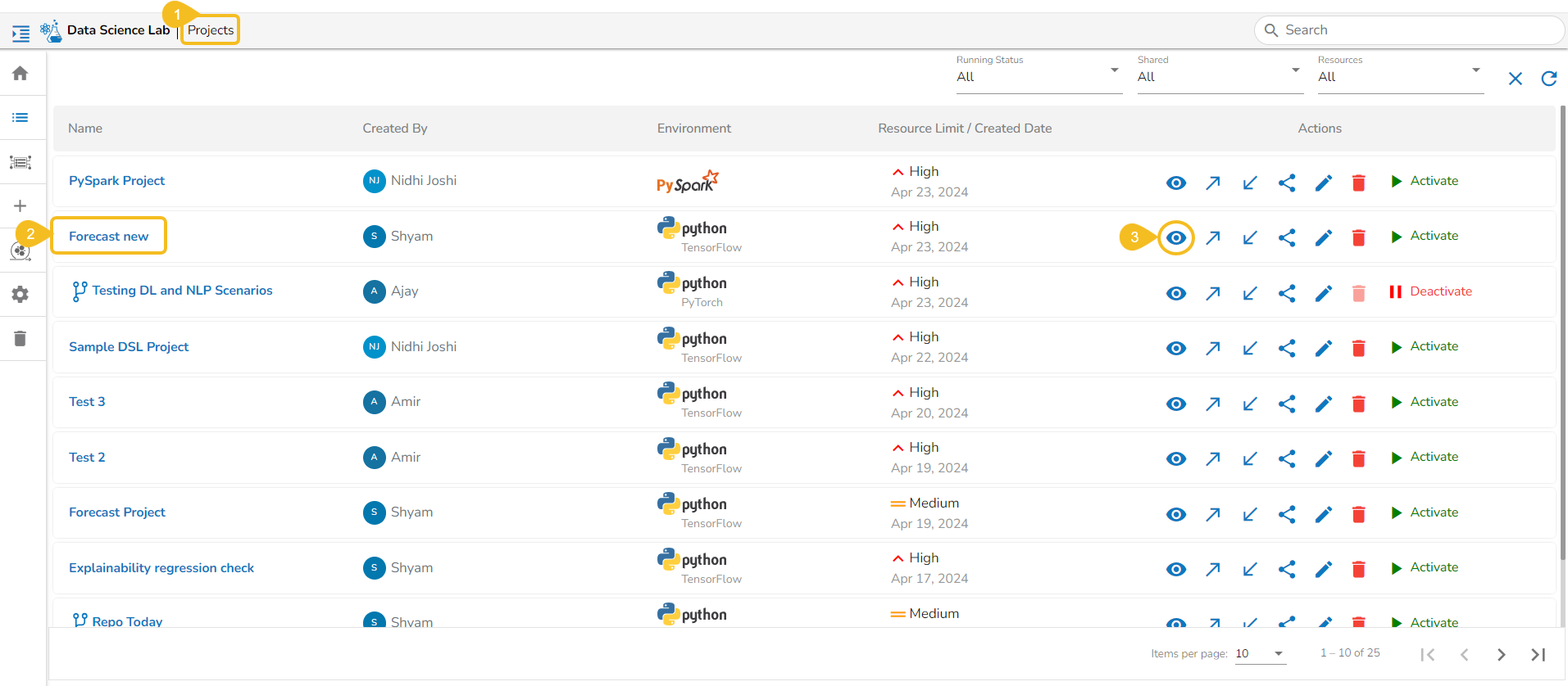
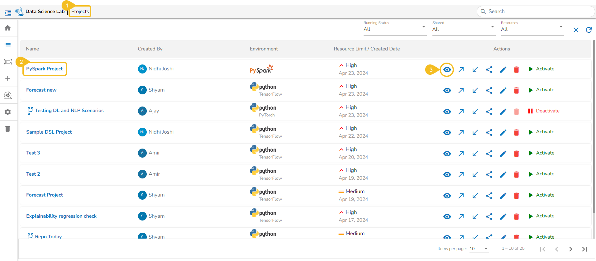
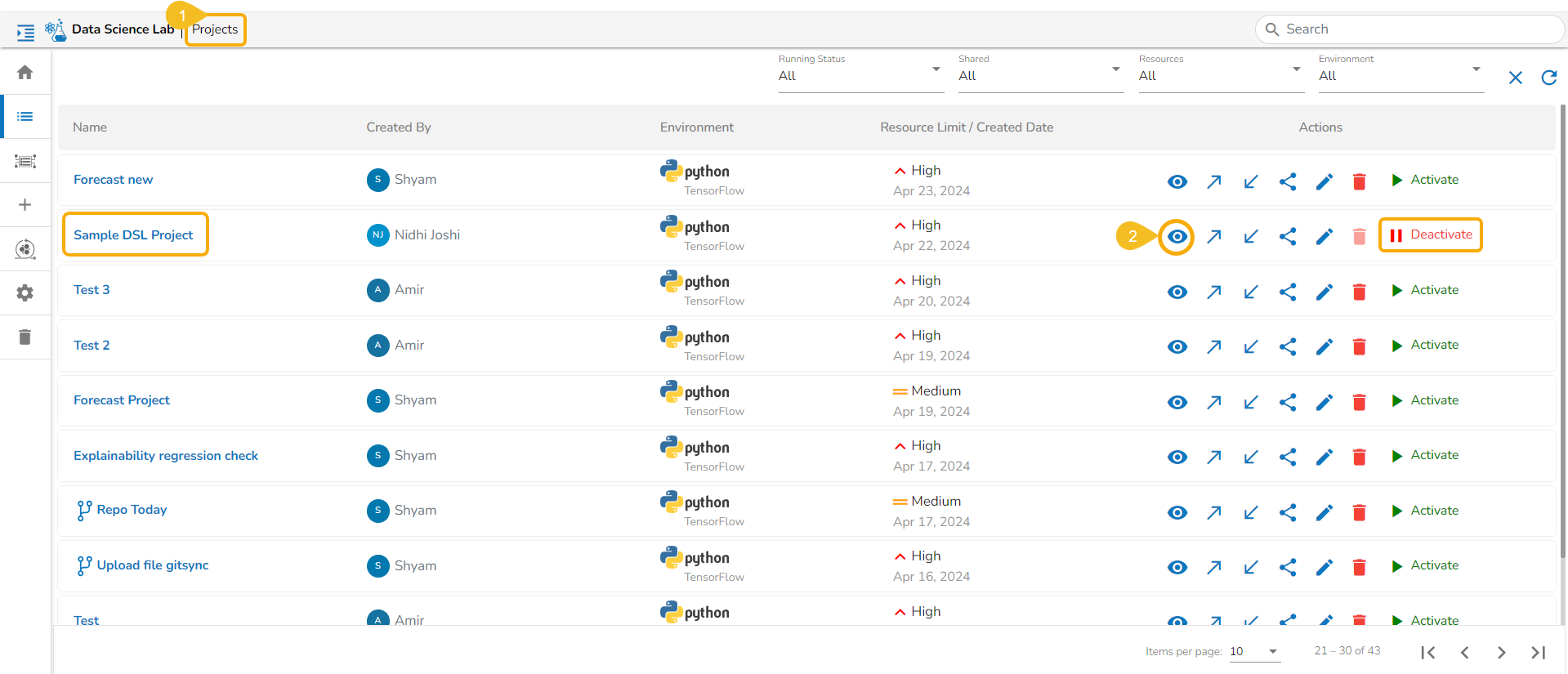
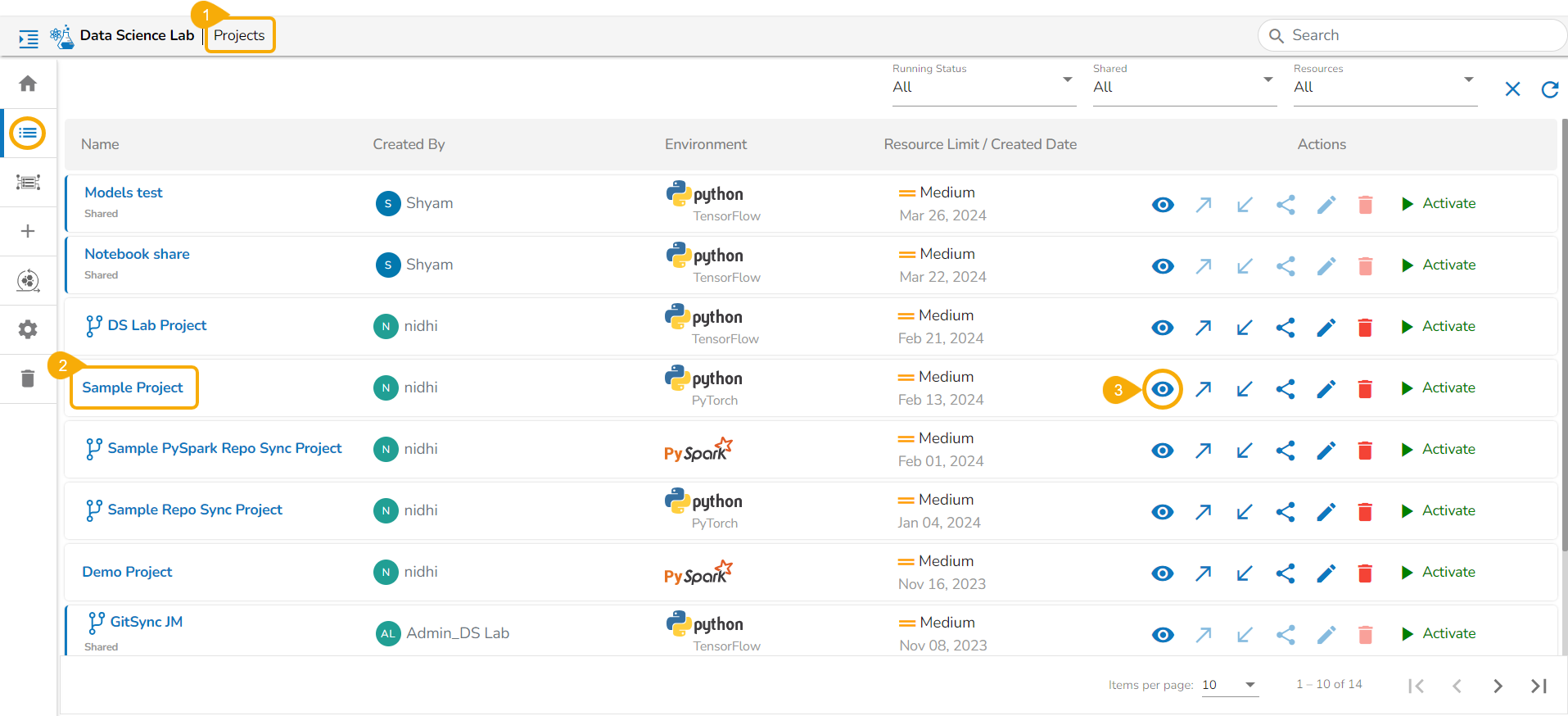
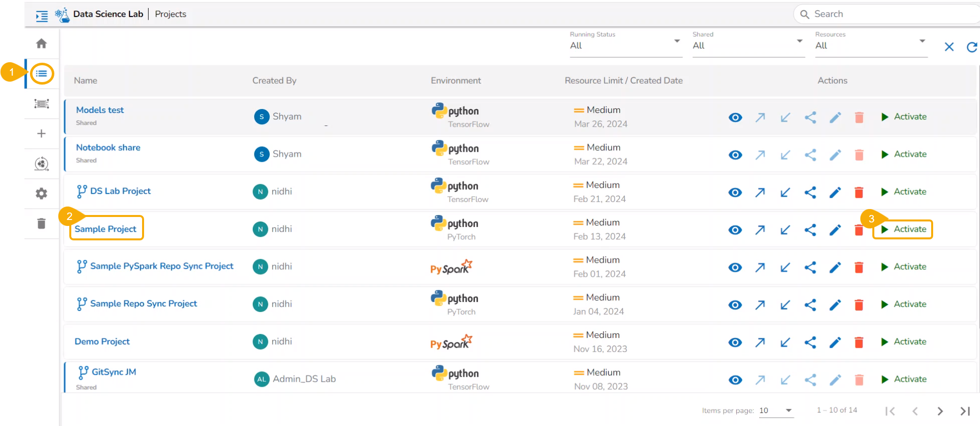
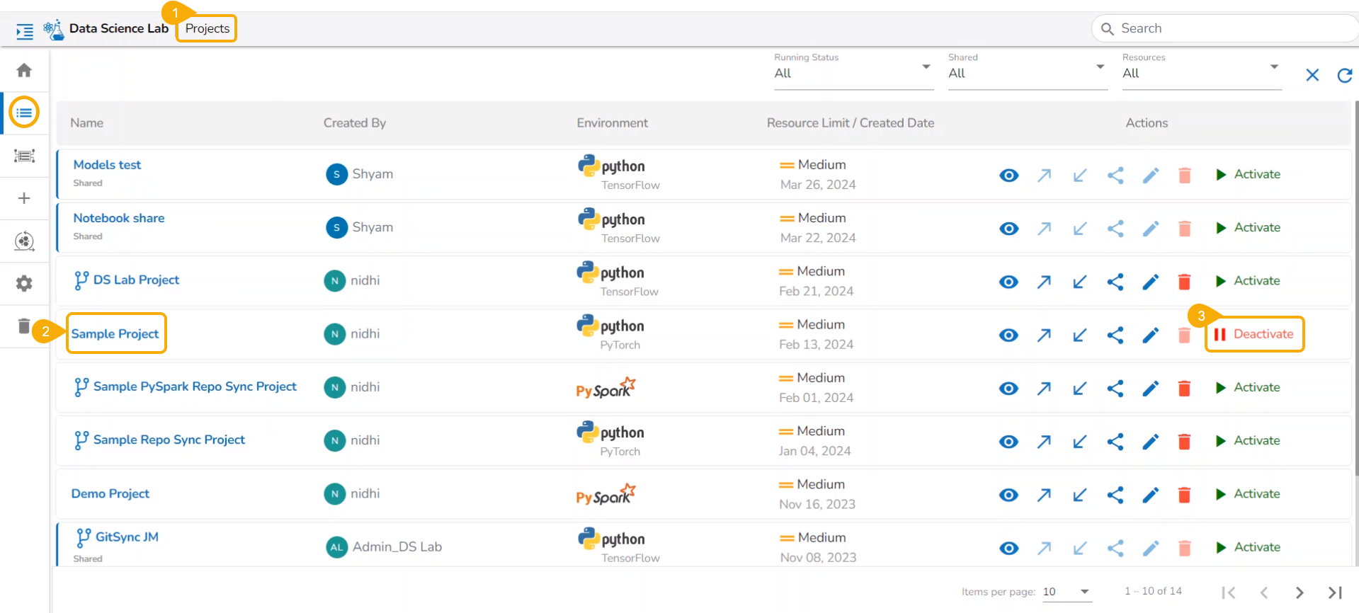
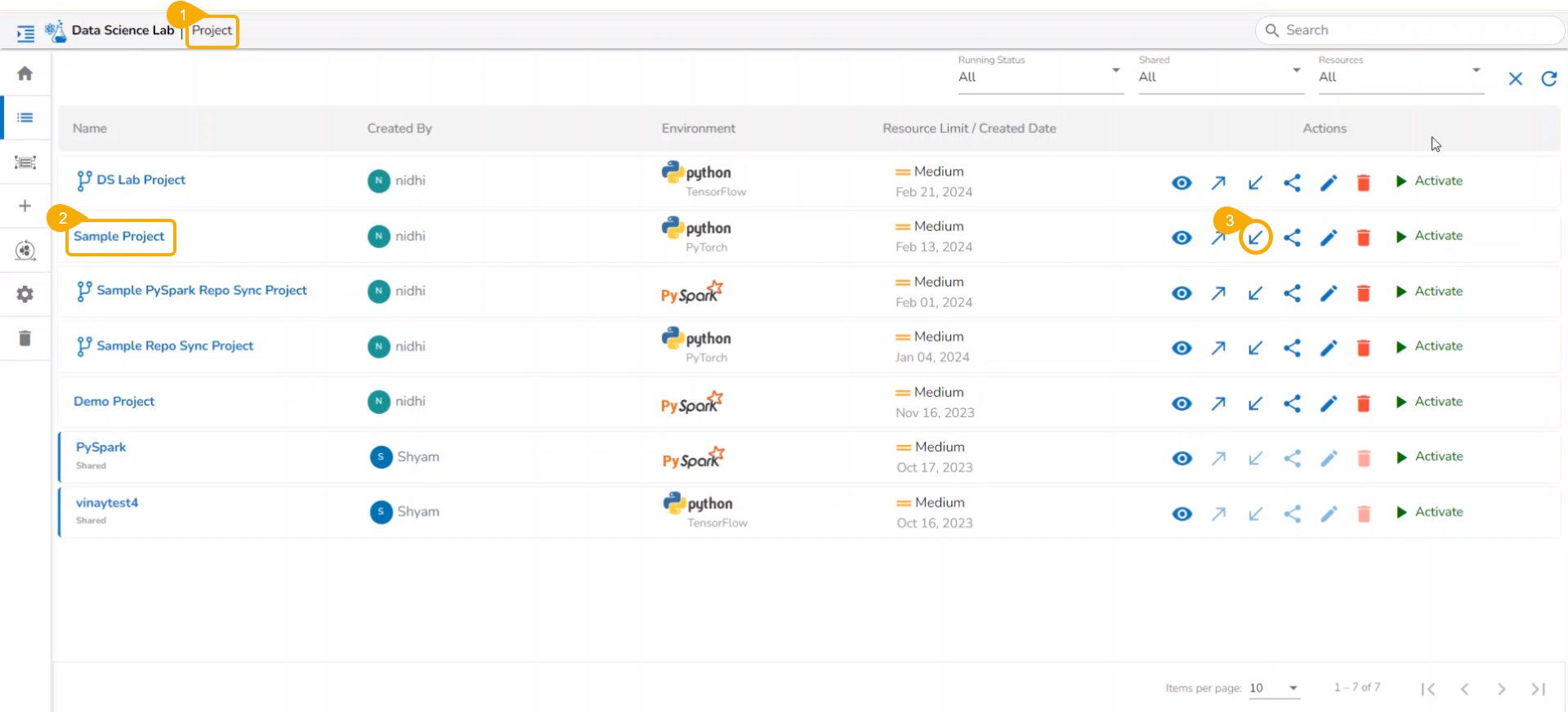
Navigate to the Project List page.
Select a deactivated Repo Sync Project from the list.
Click on the View option to open the Project.
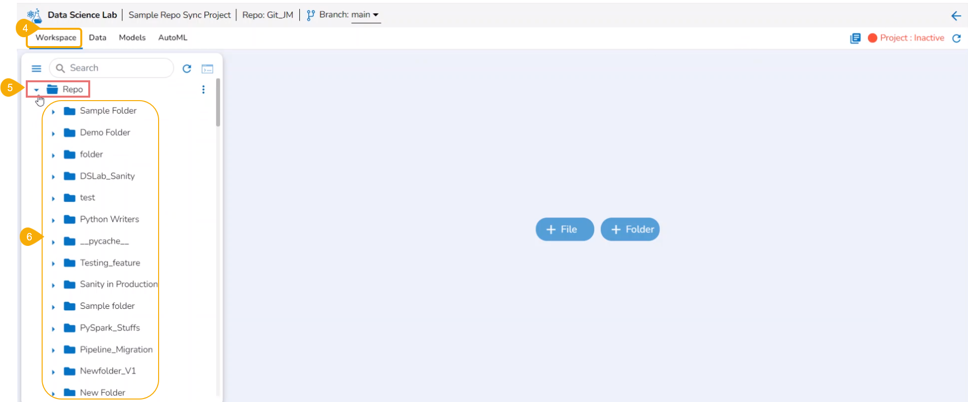
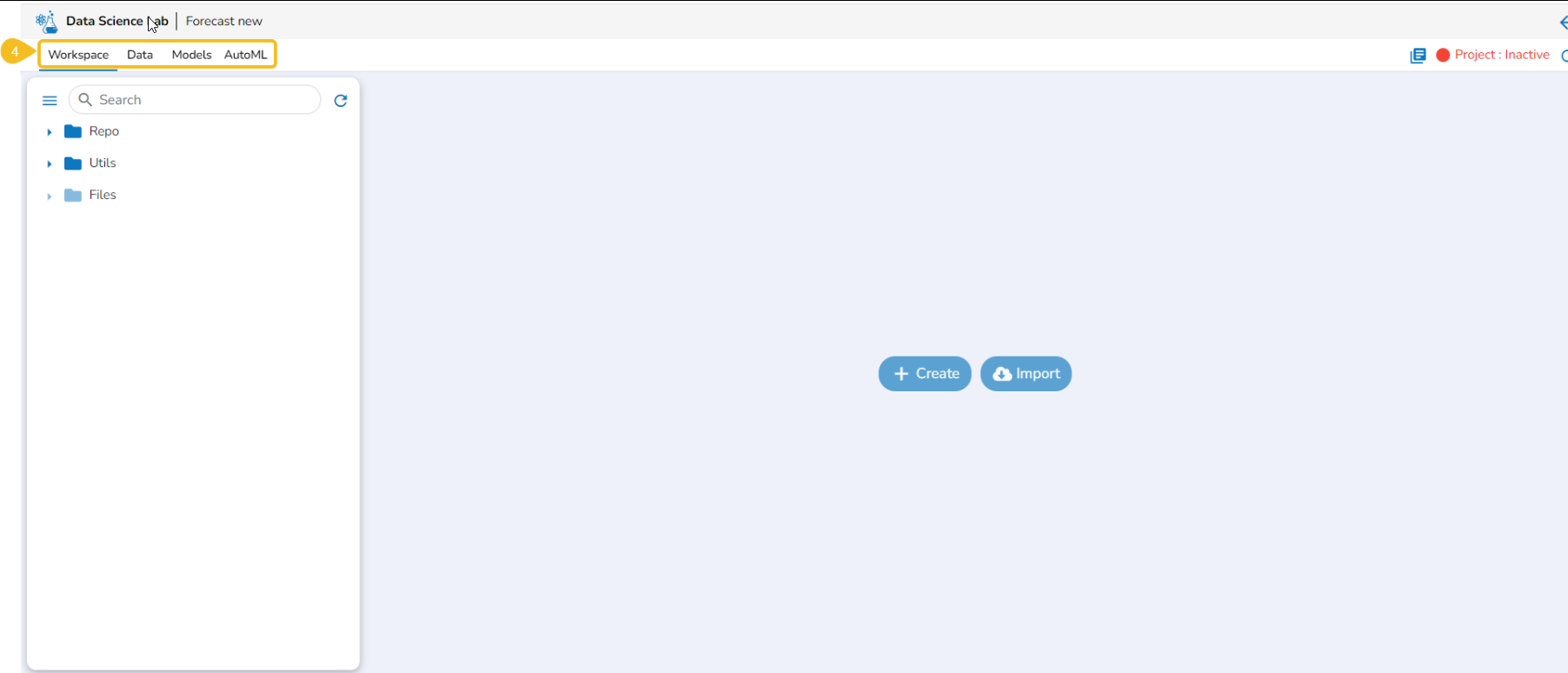
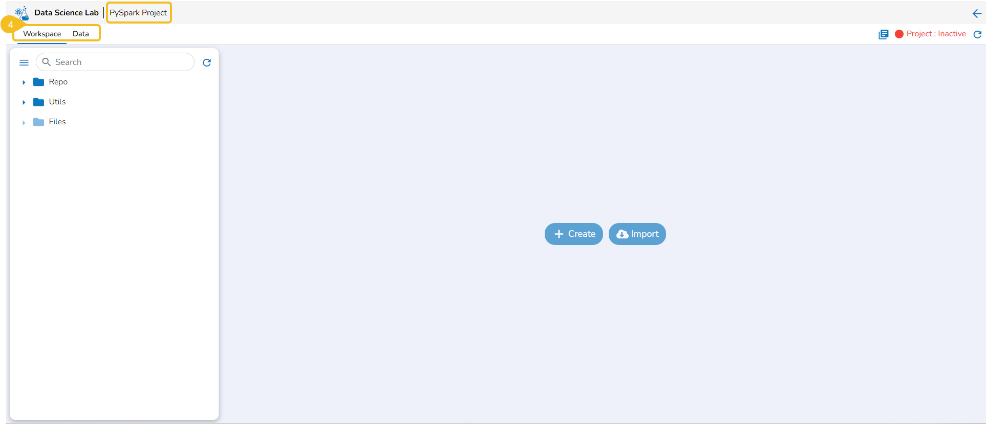
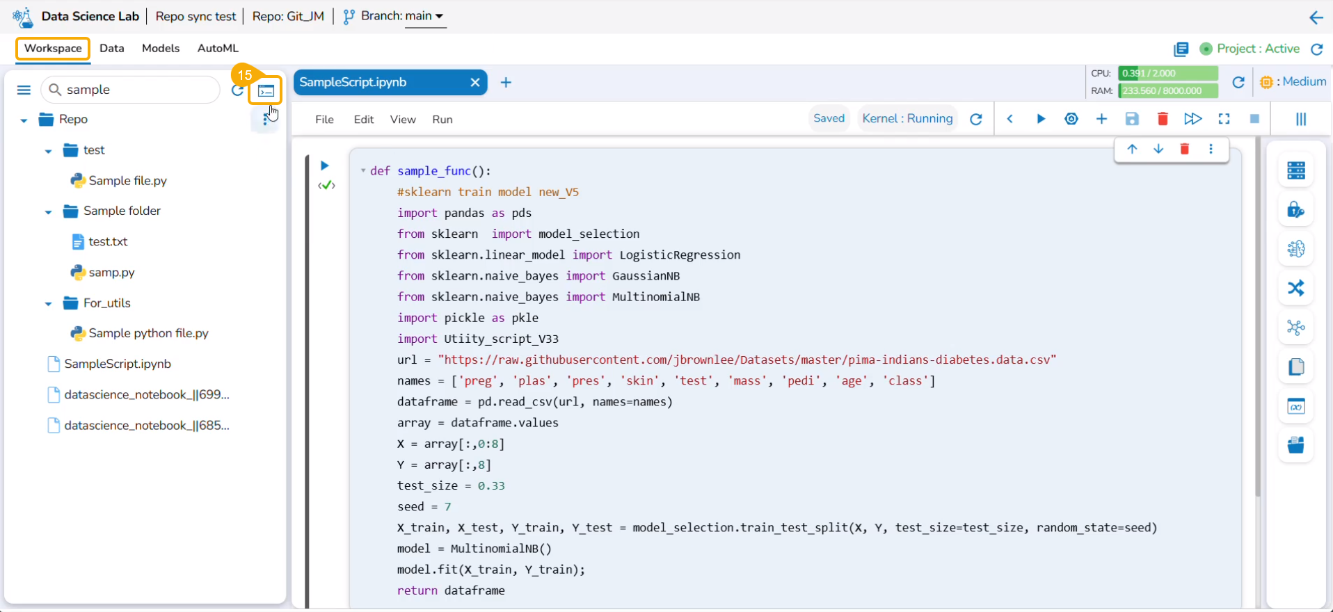
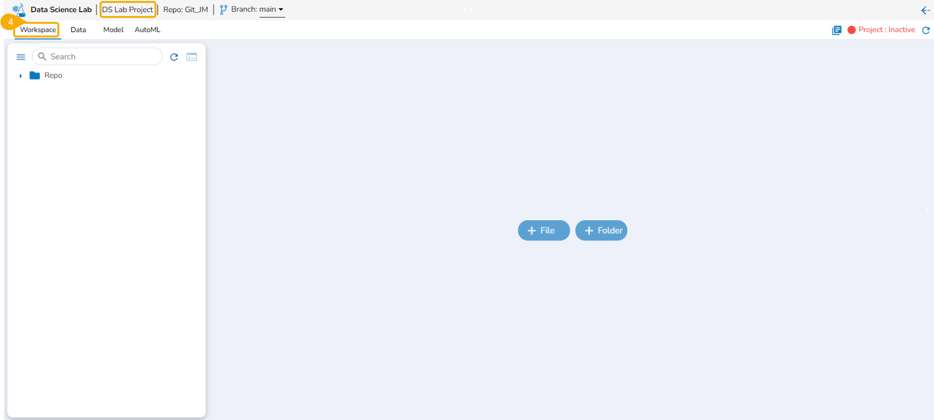
The Workspace tab opens under the selected Repo Sync Project.
Click on the Repo folder that is displayed under the Notebook tab.
A list of available folders and files appears under the Repo.
Click on a file.
The file content gets displayed.
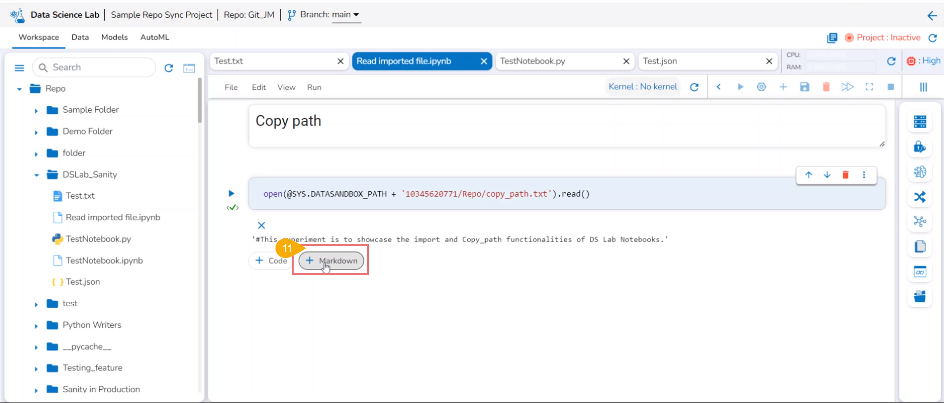
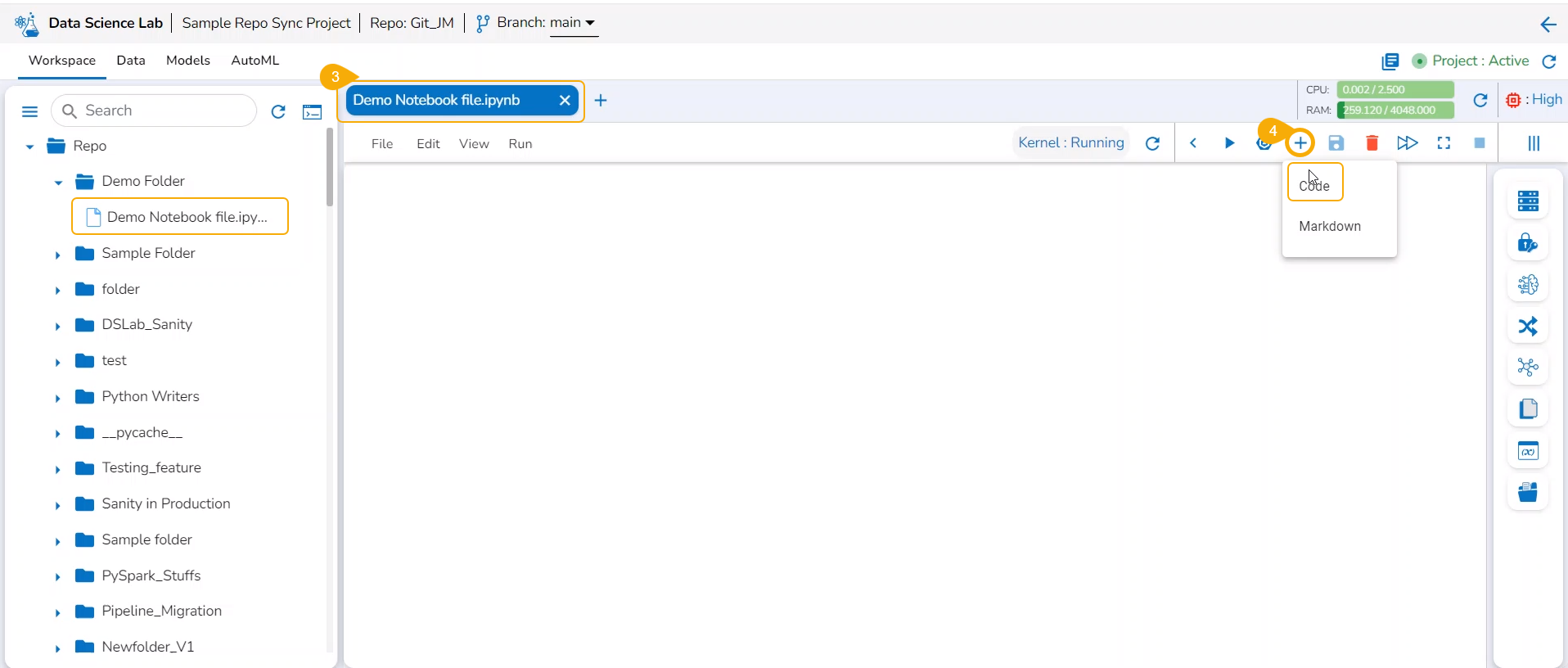
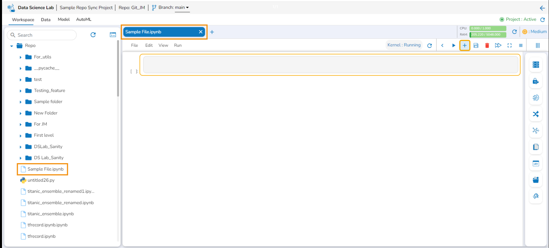
Open a .ipynb file.
The content of the file is displayed.
Click the Add code or markdown cell.
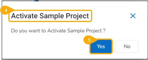
The Activate Project window opens prompting the user to activate the selected Project.
Click the Yes option from the confirmation window to activate the project. The user can choose the No option if there is no need for the project activation.
Please Note: Only Data Science Notebooks (.ipynb files) have Code, Markdown, and BDB Assist cells. The Data Science Noteboks content can be edited/ modified after activating the concerned project. The content of the other files remains in the preview category only for the activated projects as well.
Explainer Generator
This page explains how a model explainer can be generated through a job.
The user can generate an explainer dashboard for a specific model using this functionality.
Check out the illustration on Explainer as a Job.
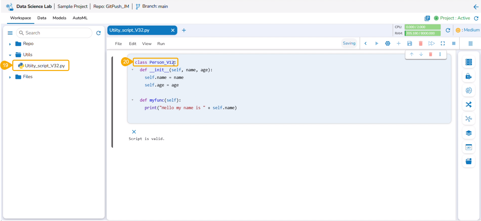
Navigate to the Workspace tab.
Open a Data Science Notebook (.ipynb file) that contains a model.
Navigate to the code cell containing the model script.
Check out the Model name. You may modify it if needed.
Click the Models tab.
The Exit Page dialog box opens to save the notebook before redirecting the user to the Models tab.
Click the Yes option.
A notification message ensures that the concerned Notebook is saved. The user gets redirected to the Models tab.
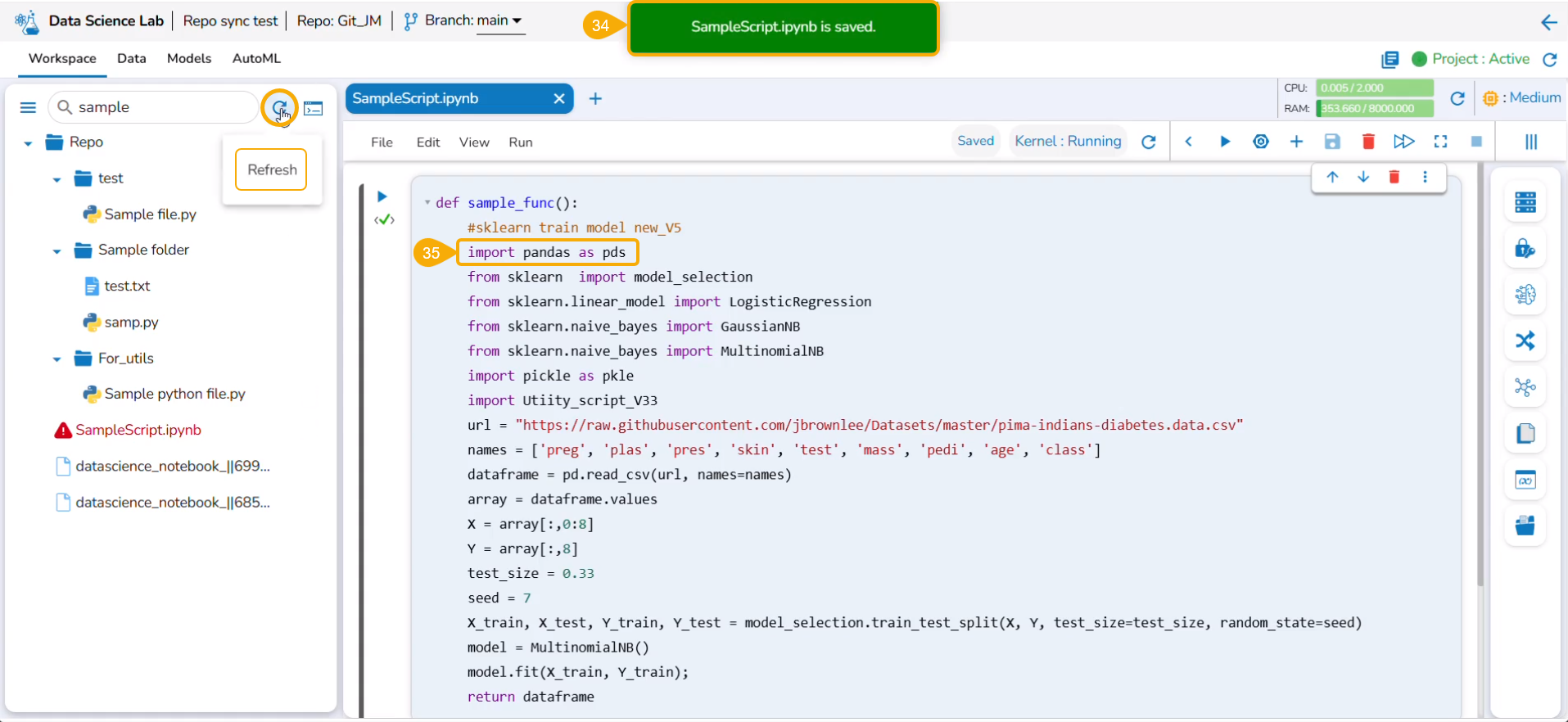
Click the Refresh icon to refresh the displayed model list.
The model will be listed at the top of the list. Click the Explainer Creator icon.
A notification ensures that a job is triggered.
Click the Refresh icon.
The Explainer icon is enabled for the model. Click the Explainer icon.
The Explainer dashboard for the model opens.
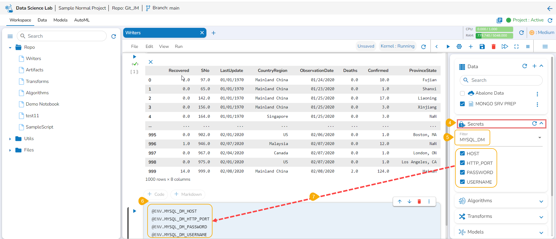
Writers
This page explains the Writers tab available in the right-side panel of the Data Science Notebook.
The Data Science Lab module provides a Writers tab inside the Notebook to write the output of the data science experiments.
Check out the illustration on how to use the Writers operation inside a DS Notebook.
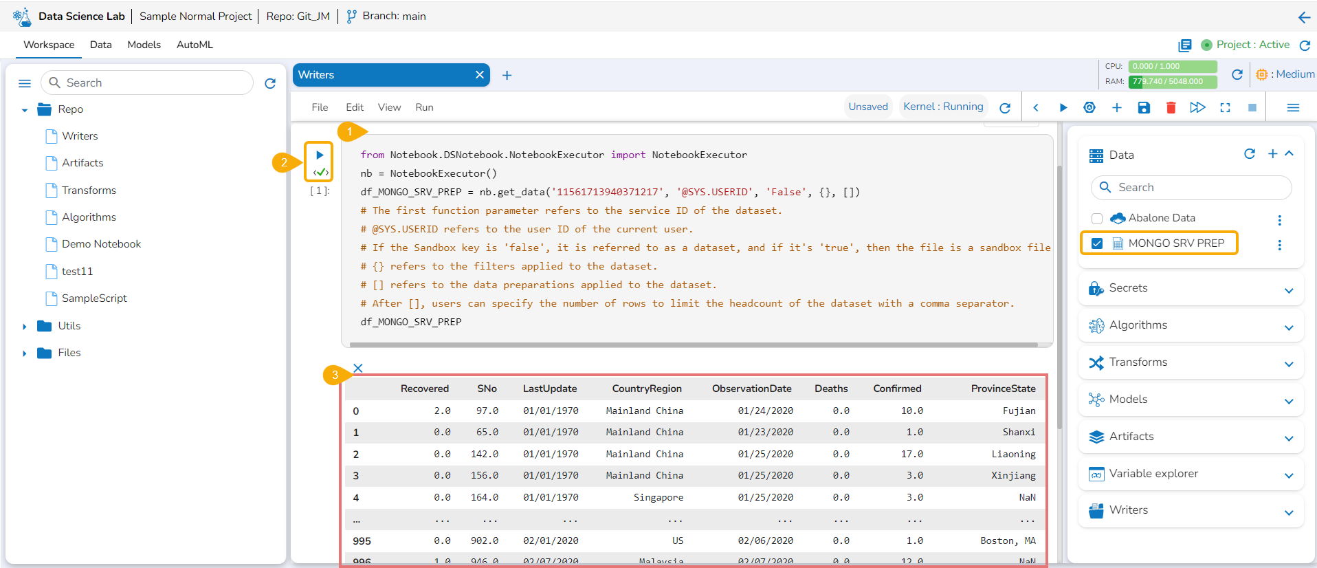
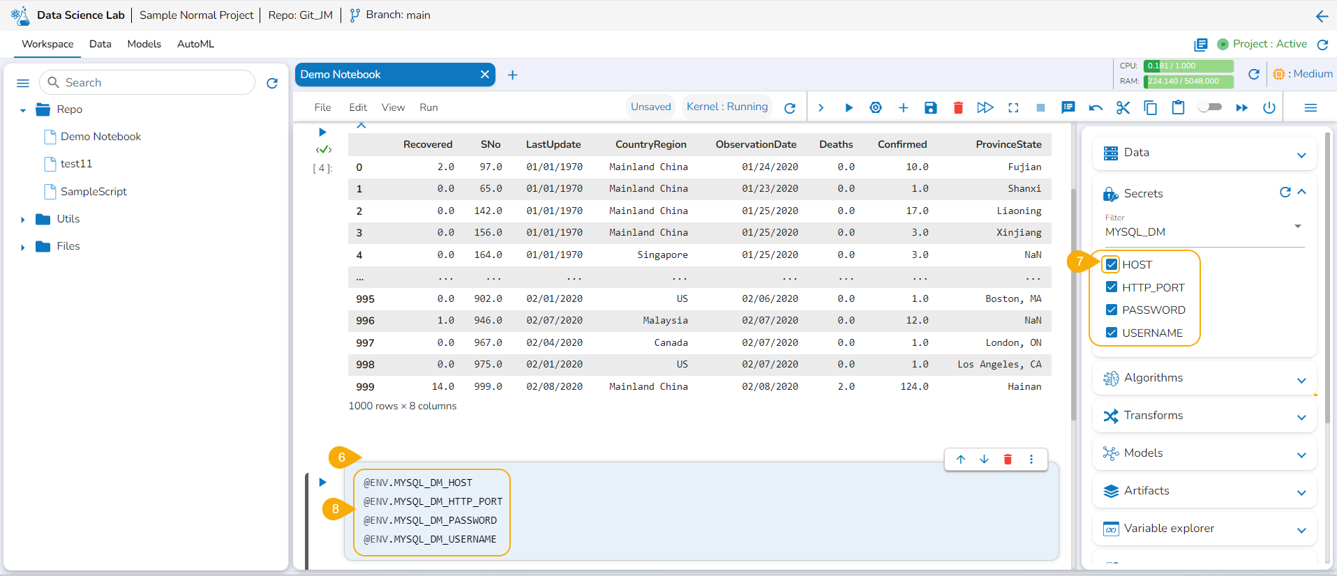
Navigate to a code cell with dataset details.
Run the cell.
The preview of the dataset appears below.
Click the Secrets tab to get the registered DB secrets.
Select the registered DB secret keys from the Secrets tab.
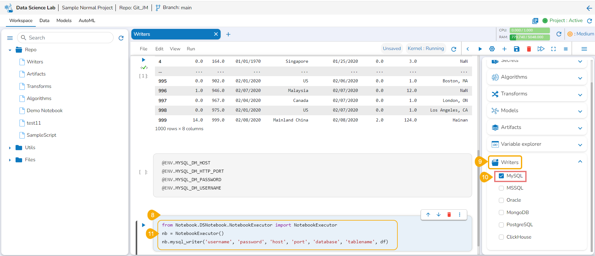
Add a new code cell.
Add a new code cell.
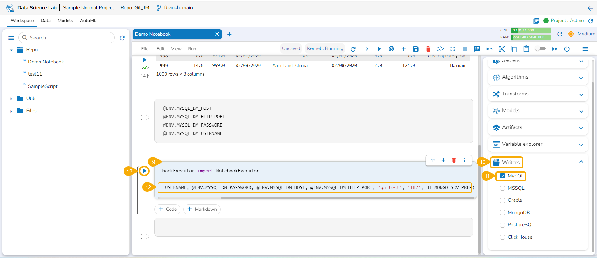
Open the Writers section.
Use the given checkbox to select a driver type for the writers.
Provide the Secret values for the required information of the writer such as Username, Password, Host, Port, Database name, table name, and DataFrame.
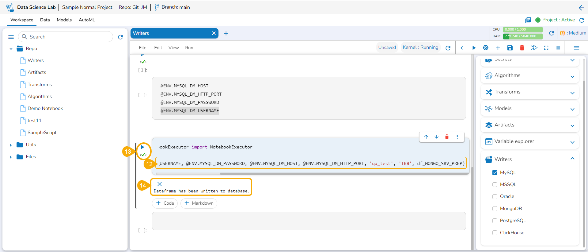
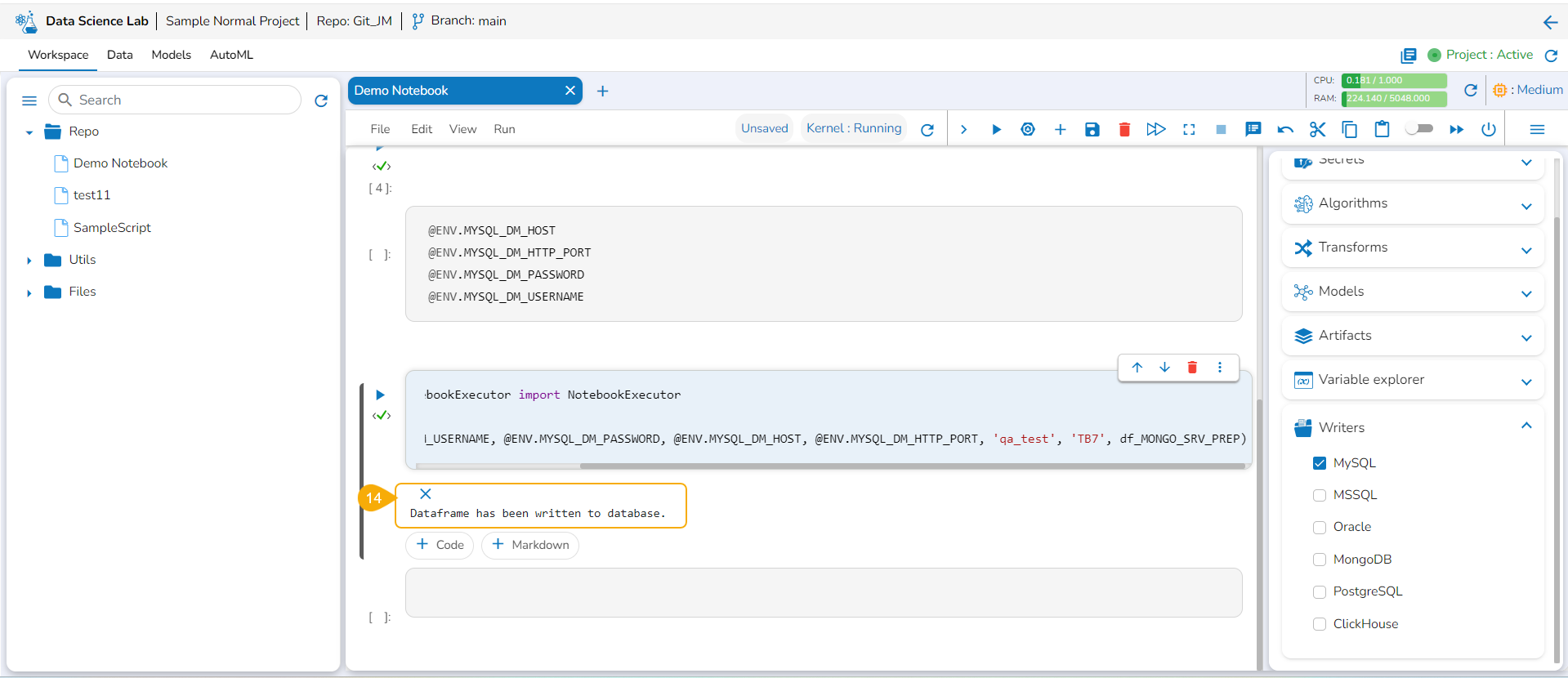
Run the code cell with the modified database details.
A message below states that the DataFrame has been written to the database. The data gets written to the specified database.
Please Note:The supported DB writers are MYSQL, MSSQL, Oracle, MongoDB,PostgreSQL, and ClickHouse.
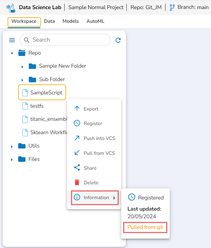
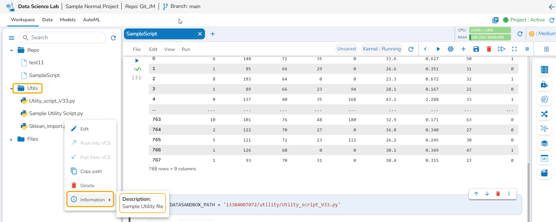
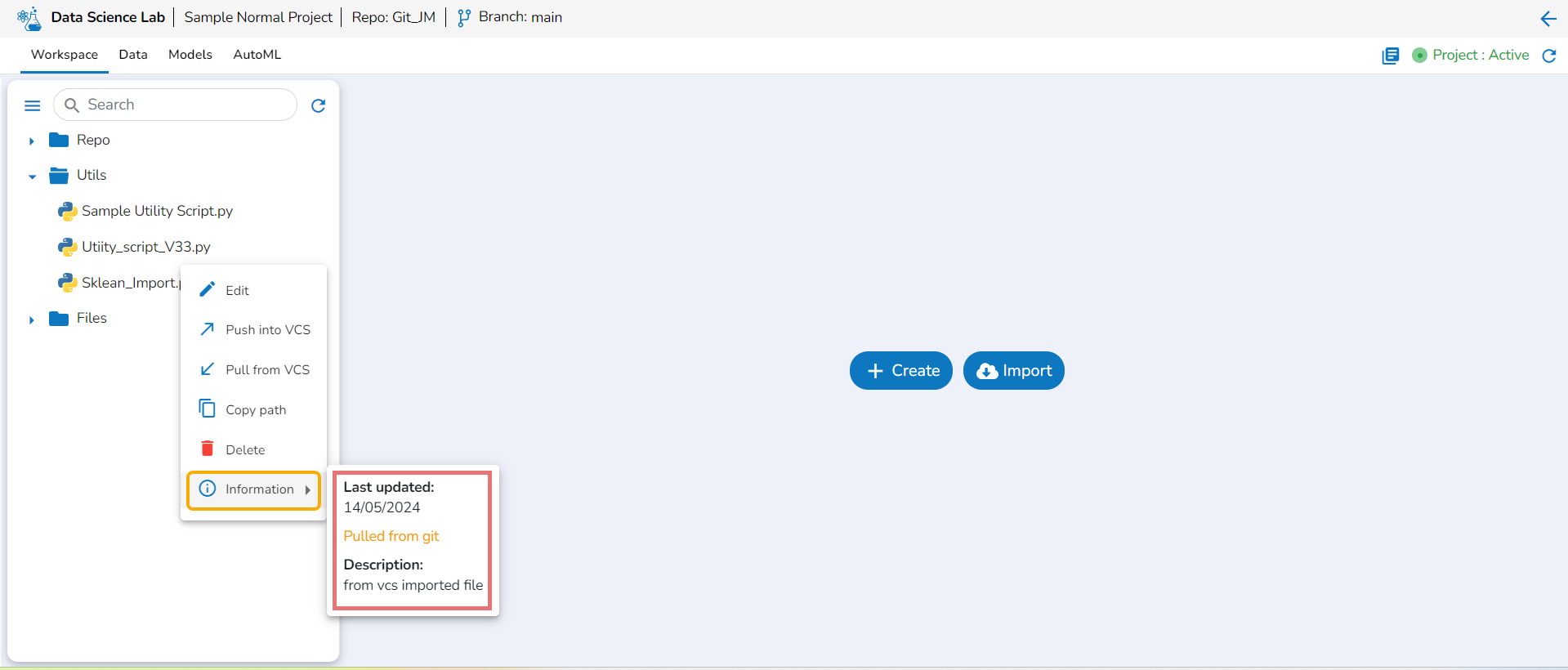
Information
This option displays the last modified date for the selected notebook.
Navigate to the Workspace tab.
Open the Repo folder.
Select a notebook from the Repo folder and click the ellipsis icon for the selected notebook.
A Context Menu opens. Select the Information option from the Context Menu.
The last modified date for the selected notebook is displayed.
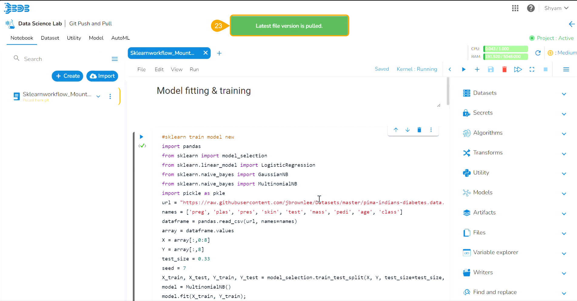
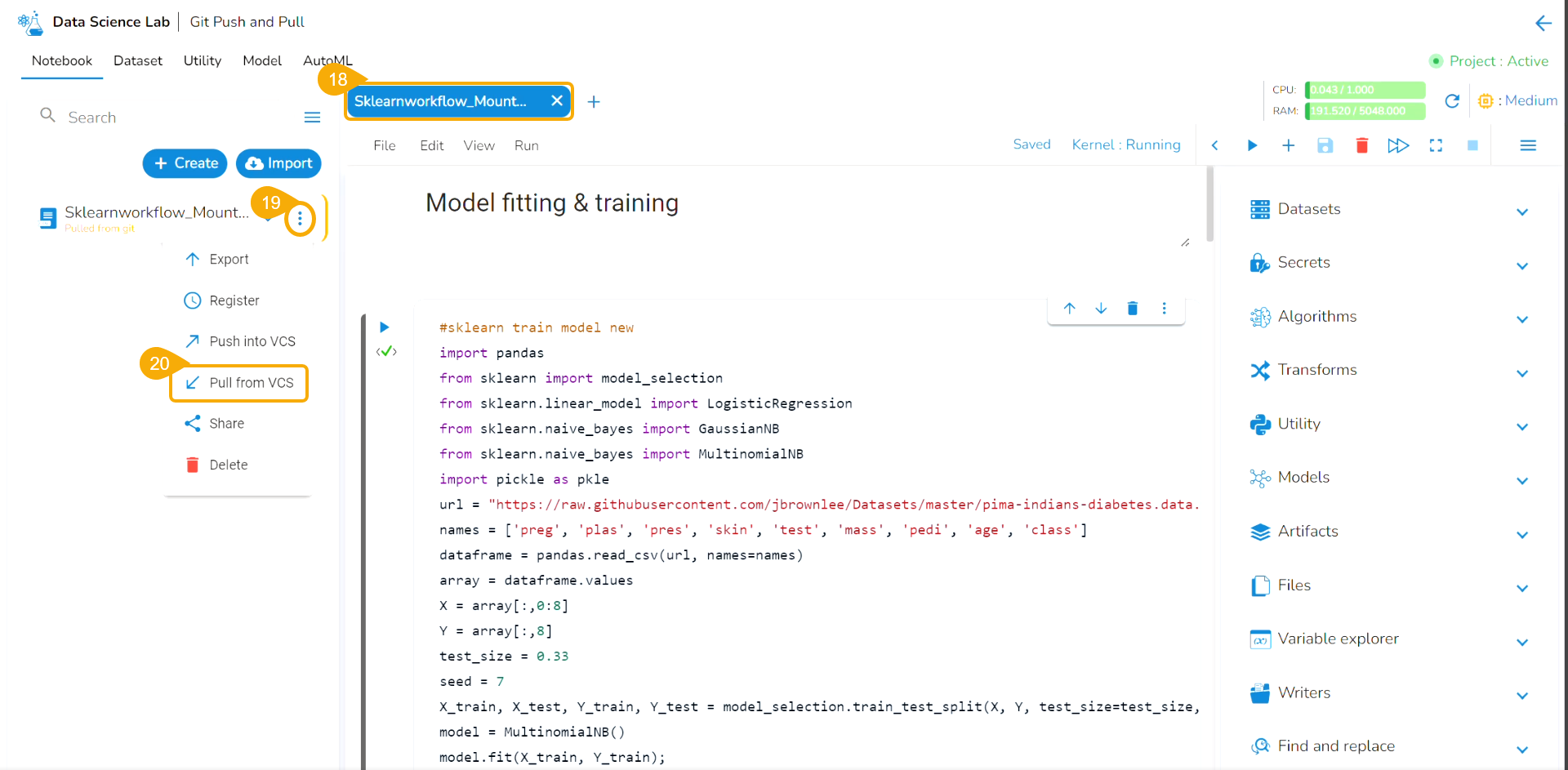
The Notebooks pulled from Git get 'Pulled from git' mentioned inside the Information Context menu.
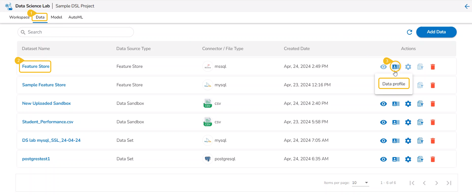
List Feature Stores
This page focuses on the Feature Store List Actions.
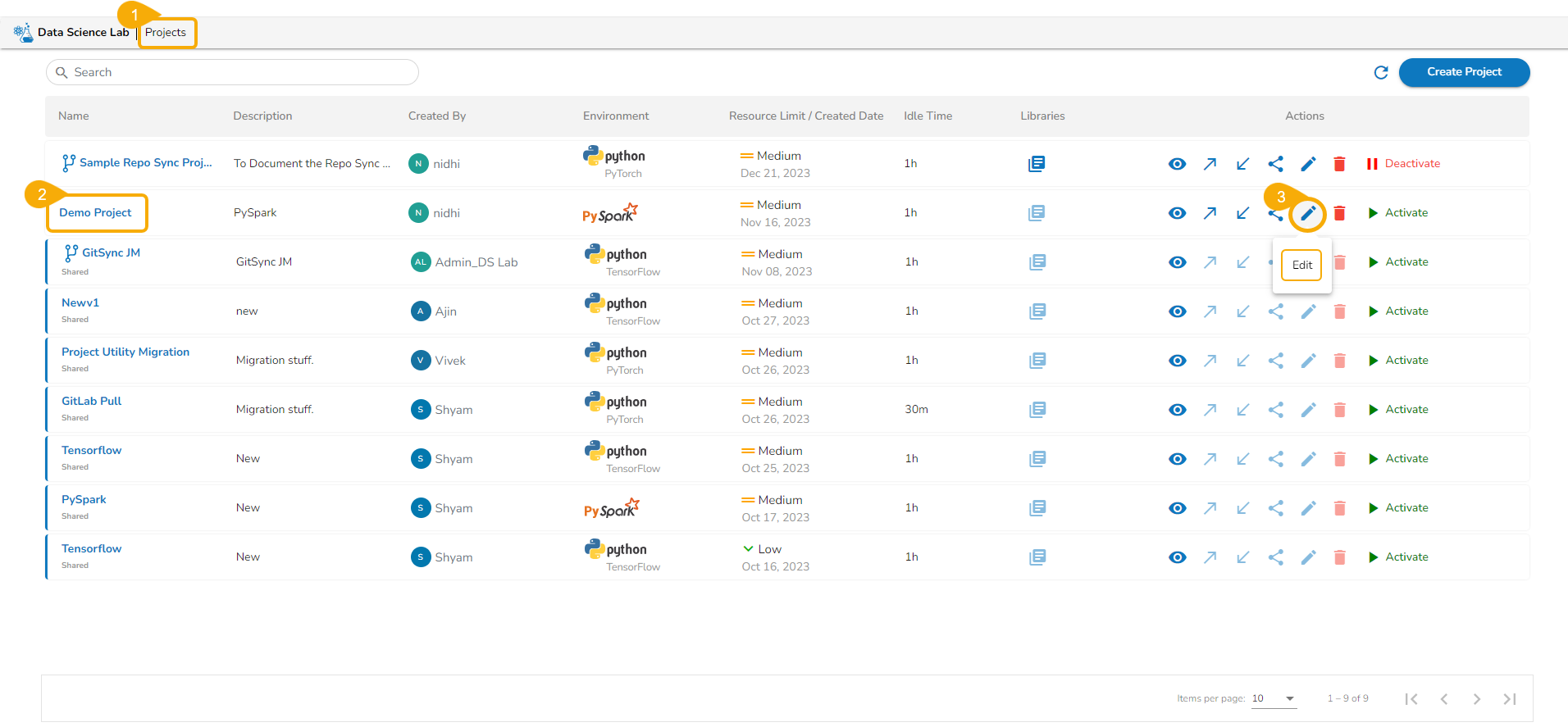
Editing a Feature Store
Check out the illustration to understand the steps to edit a feature store.
Repo Folder Attributes
The Repo folder is a default folder created under the Workspace tab. It opens by default while accessing the Workspace tab.
The user can perform some attributive actions on the Repo folder using the ellipsis icon provided next to it. This page explains all the attributes given to the Repo folder. This folder contains only .ipynb files in it. The actions provided for a .ipynb file (Notebook) are mentioned under the page.
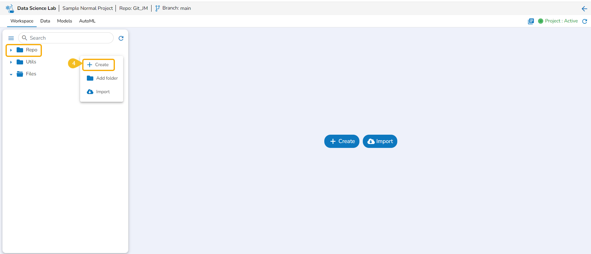
Create
This option redirects the user to the Create Notebook page to create a new Notebook.
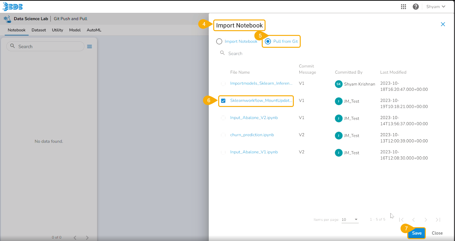
Importing Notebook
You can bring your Python script to the Notebook framework to carry forward your Data Science experiment.
Please Note: The Import option appears for the Repo folder.
The Import functionality contains two ways to import a Notebook.
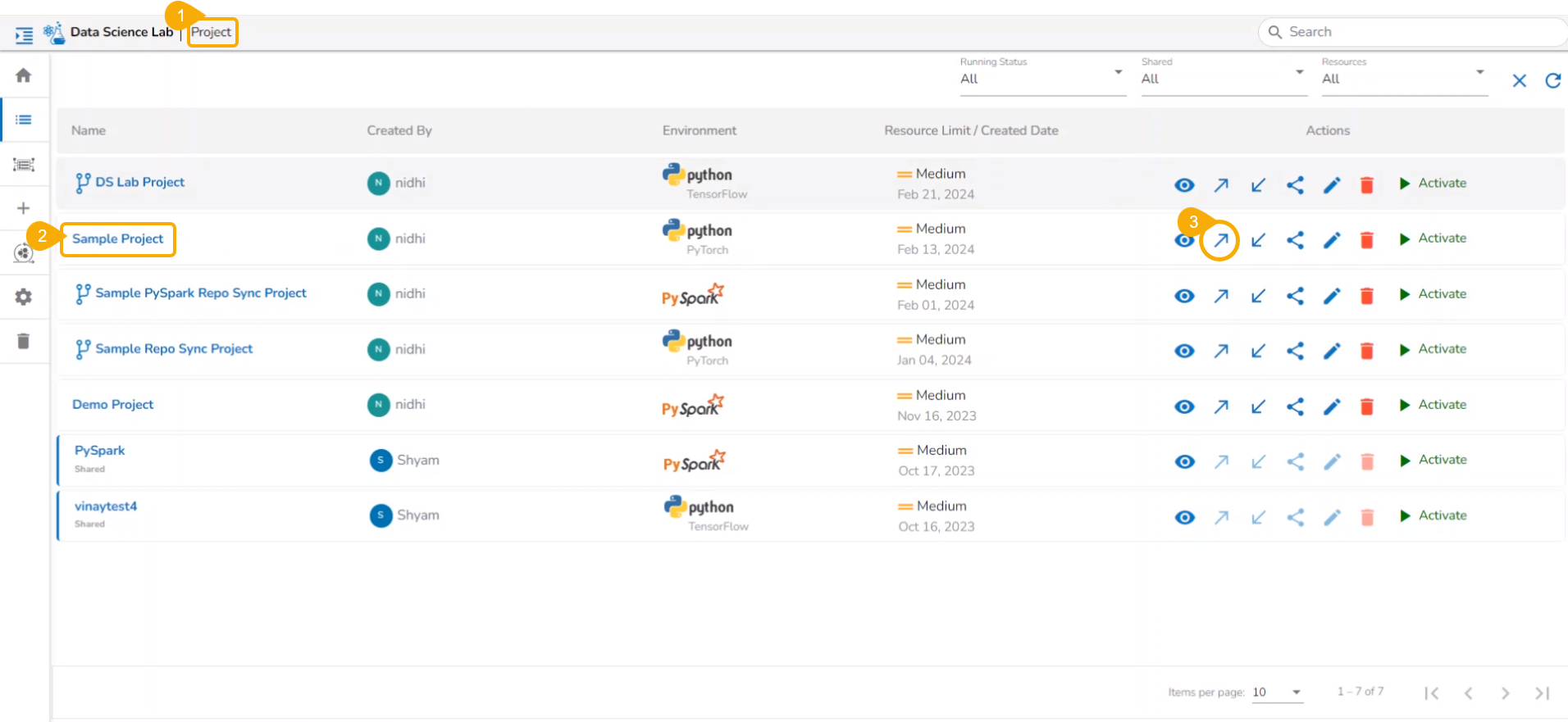
Tabs for a DSL Project
A DSL project utilizes tabs to structure a data science experiment, enabling the outcome to be readily consumed for further data analytics.
How to access the Tabs?
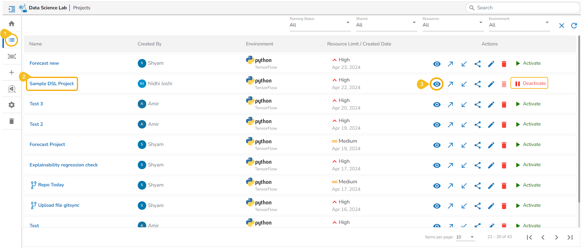
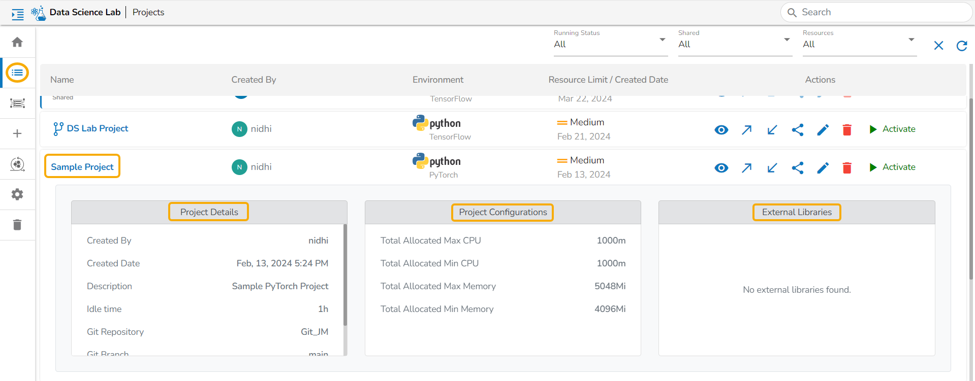
The users can click on the View icon available for a DSL Project, it redirects to a page displaying the various tabs for the selected DSL Project.
Navigate to the
Workspace
The Workspace is a placeholder to create and save various data science experiments inside the Data Science Lab modules.
The Workspace is the default tab to open for each Data Science Lab project. Based on the Project types the options to begin working with Workspace may differ.
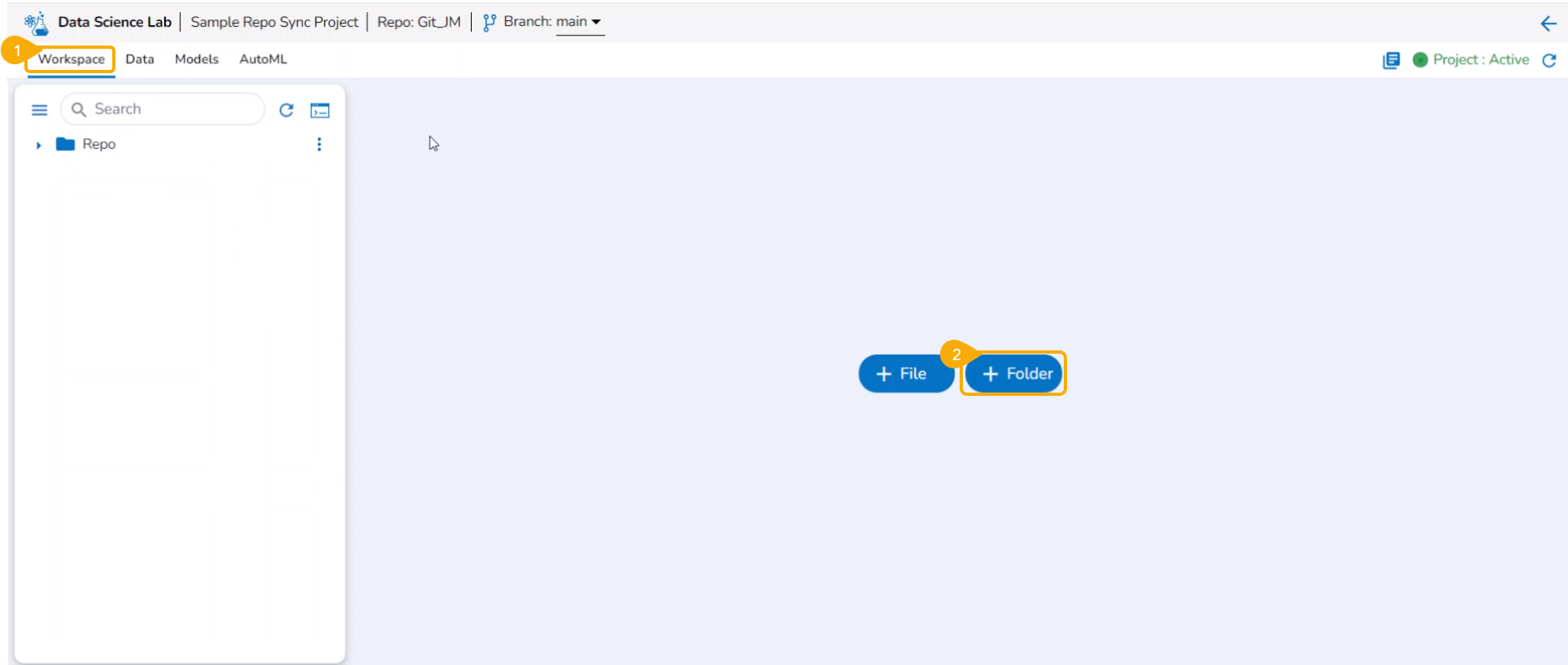
The Repo Sync Projects offer File and Folder options on the default page of the Workspace tab.
The normal Data Science Projects will have Create and
Model Creation using Data Science Notebook
This section aims to step down the process of creating, saving, and loading a Data Science model using the notebook infrastructure provided inside the Data Science Lab module.
Once the Notebook script is executed successfully, the users can save them as a model. The saved model can be loaded into the Notebook.
Check out the illustration on saving and loading a Data Science Model.
Artifacts
This page explains how to save Artifacts. Users can save plots and datasets inside a DS Notebook as Artifacts.
Check out the walk-through on how to Save Artifacts.
Saving Artifacts
Variable Explorer
Get the Variables information listed under this tab.
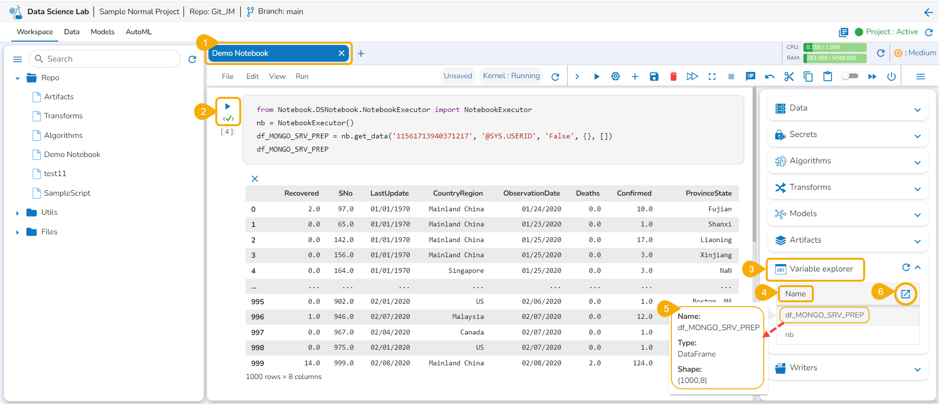
The Variable Explorer tab displays the Name column and Explore icon for all the variables created and executed within the Notebook cells.
Navigate to the Notebook page.
Write and run code using the Code cells.
Transforms: Save and load models with transform script, register them, or publish them as an API through the DS Lab module.
Models: You can train, save, and load the models (Sklearn, Keras/TensorFlow, PyTorch). You can also register a model using this tab. Refer to Model Creation using Data Science Notebookfor more details.
Artifacts: You can save the plots and datasets as Artifacts inside a DS Notebook.
Variable Explorer: Get detailed information on Variables declared inside a Notebook.
Writers: Write the DSL experiments' output into the database writers' supported range.
Click the Choose File option to import a utility file.
Click once for the first level, twice for the second, and thrice for the third.
Unassigned Markdown cells default to the nearest existing hierarchy.
Remember to click Save to preserve changes.
The Markdown cell will get a collapse/expand icon added to it.
Get the Secret keys of the DB using the checkboxes provided for the listed Secret keys.
The code gets added to the newly added cell.
Navigate to the Feature Stores page.
Select a Feature Store from the list.
Click the Edit icon for the selected Feature Store.
The EditFeature Store form opens.
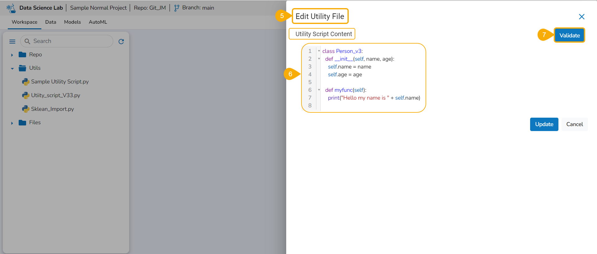
Modify the required information.
Click the Validate option for the Feature Store.
A notification message ensures that the action updating table is executed.
The data preview is displayed below.
Click the Update option after getting a notification message for successful validation.
Another notification message appears to ensure that the updated Feature Store is saved.
Use the Refresh icon provided on the Feature Stores list.
The status of the updated Feature Store will be listed in the Feature Stores list.
Click the Refresh icon again till the Feature Store status turns Completed.
The Version column will display the version number, indicating that the Feature Store has been updated.
Updated Feature Store
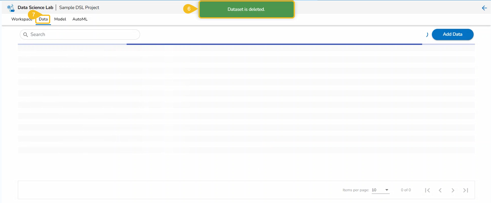
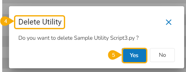
Deleting a Feature Store
Check out the illustration to understand the steps to delete a feature store.
Navigate to the Feature Stores List page.
Select a Feature Store from the list. Select a Feature Store with more than one version with Status marked as Completed.
It will display all the available versions of the selected Feature Store.
Click the Delete icon for a version of the selected Feature Store you wish to delete.
Multiple Versions of the Feature Store
The Delete confirmation dialog box appears.
Click the Yes option.
A notification message appears to inform the user about the deletion.
The selected version of the Feature Store will be removed, but another version will be listed in the Feature Stores List.
Please Note: The Feature Store with only one version, gets removed from the Feature List.
The deleted Feature Store version can be accessed from the Trash page. The user can restore it or delete it permanently from this page.
Deleted Feature Store version listed under the Trash page
Navigate to the Workspace tab.
Select the Repo folder.
Click the Elipsis icon.
A Context Menu appears. Select the Create option from the Context Menu.
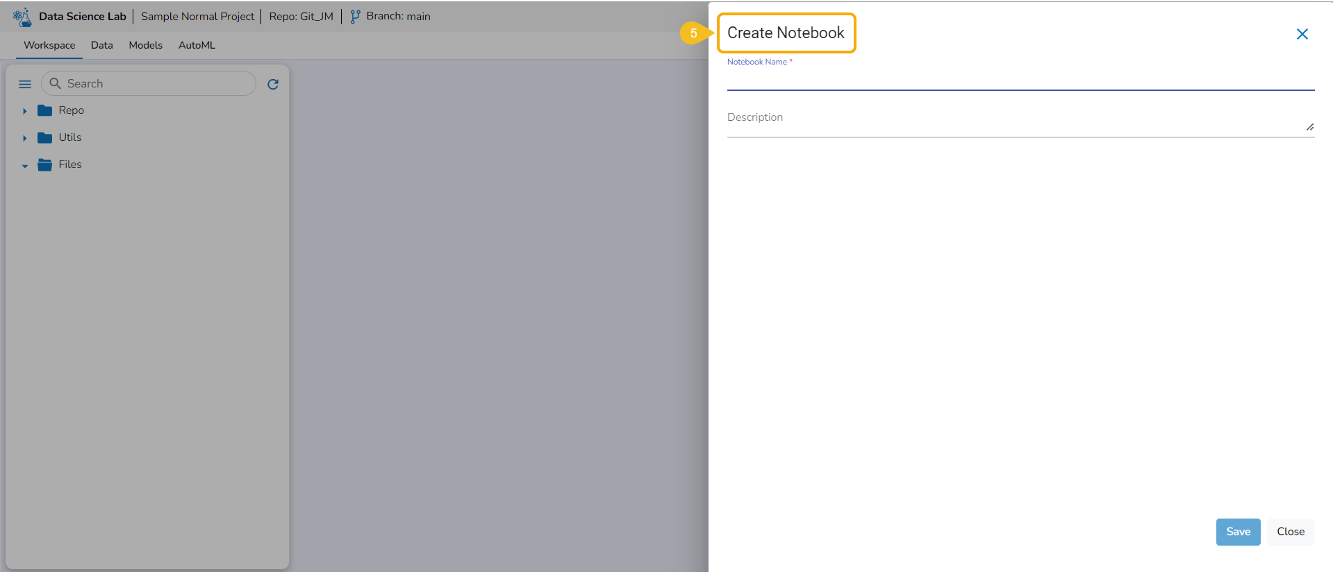
The Create Notebook drawer opens.
Please Note: Refer to the Create page to learn the steps to create a new Notebook.
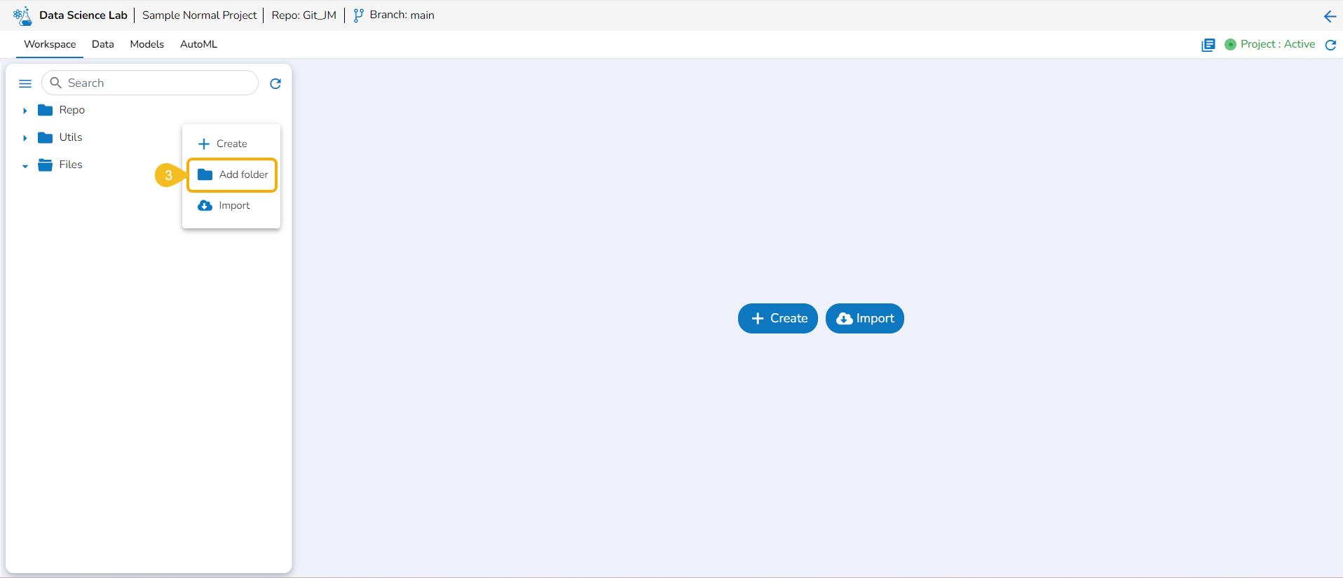
Add Folder
This option allows the user to create folders under the Repo folder.
Navigate to the Workspace tab.
Select the Repo folder.
Click the Elipsis icon.
A Context Menu appears. Select the Add Folder option from the Context Menu.
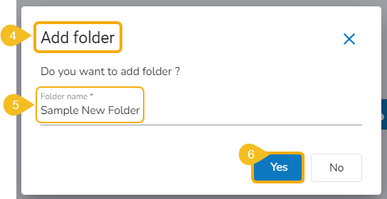
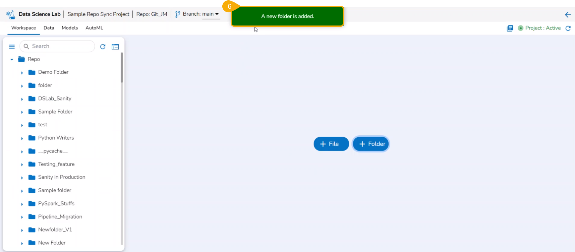
The Add folder dialog box opens.
Provide a name to the folder.
Click the Yes option.
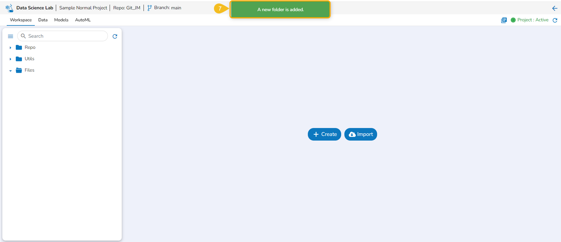
A notification appears to ensure the folder creation.
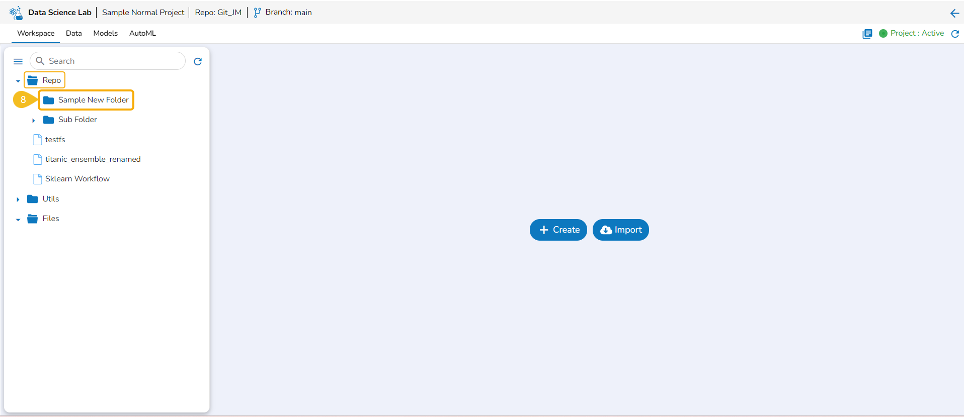
The newly added folder is listed under the Repo folder. Expand the Repo folder to see the newly added folder.
Import
The Import option allows users to import a .ipynb file to the selected Data Science Lab project from their system.
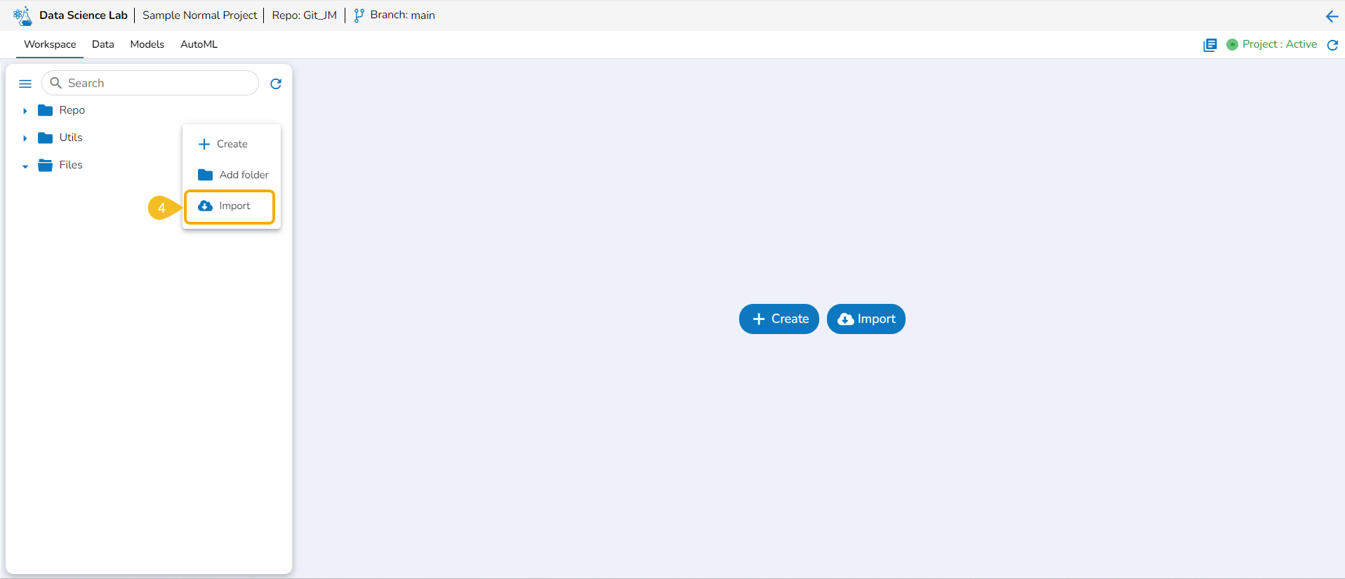
Navigate to the Workspace tab.
Select the Repo folder.
Click the Elipsis icon.
A Context Menu appears. Select the Import option from the Context Menu.
The Import Notebook page opens.
Please Note:
Refer to theImport Notebookpage to learn how to import a Notebook.
Created or Imported Notebooks will get some attributed Actions. The are described under this documentation's section.
The users can seamlessly import Notebooks created using other tools and saved in their systems.
Please Note: The downloaded files in the .ipynb format only are supported by the Upload Notebook option.
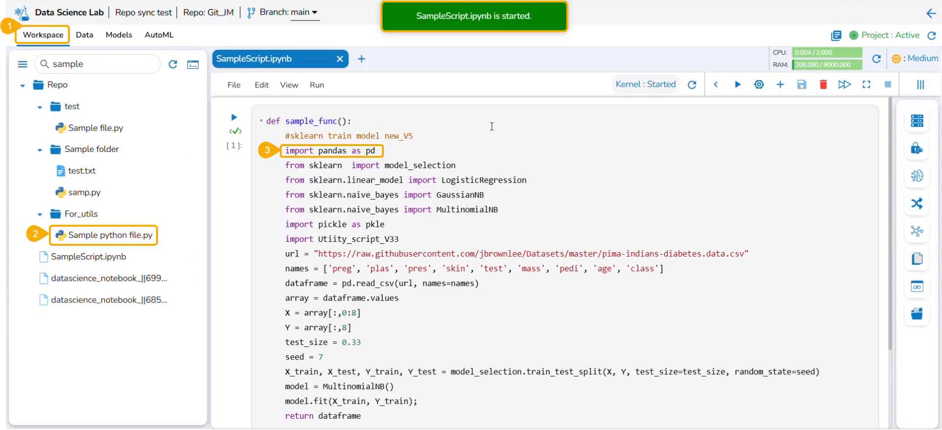
Check out the given illustration on how to import a Notebook.
Navigate to the Projects tab.
Click the View icon for an activated project.
The next page opens displaying all the related tabs.
The Workspace tab opens by default.
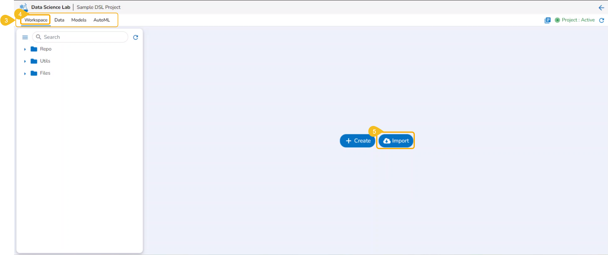
Click the Import option from the Workspace tab.
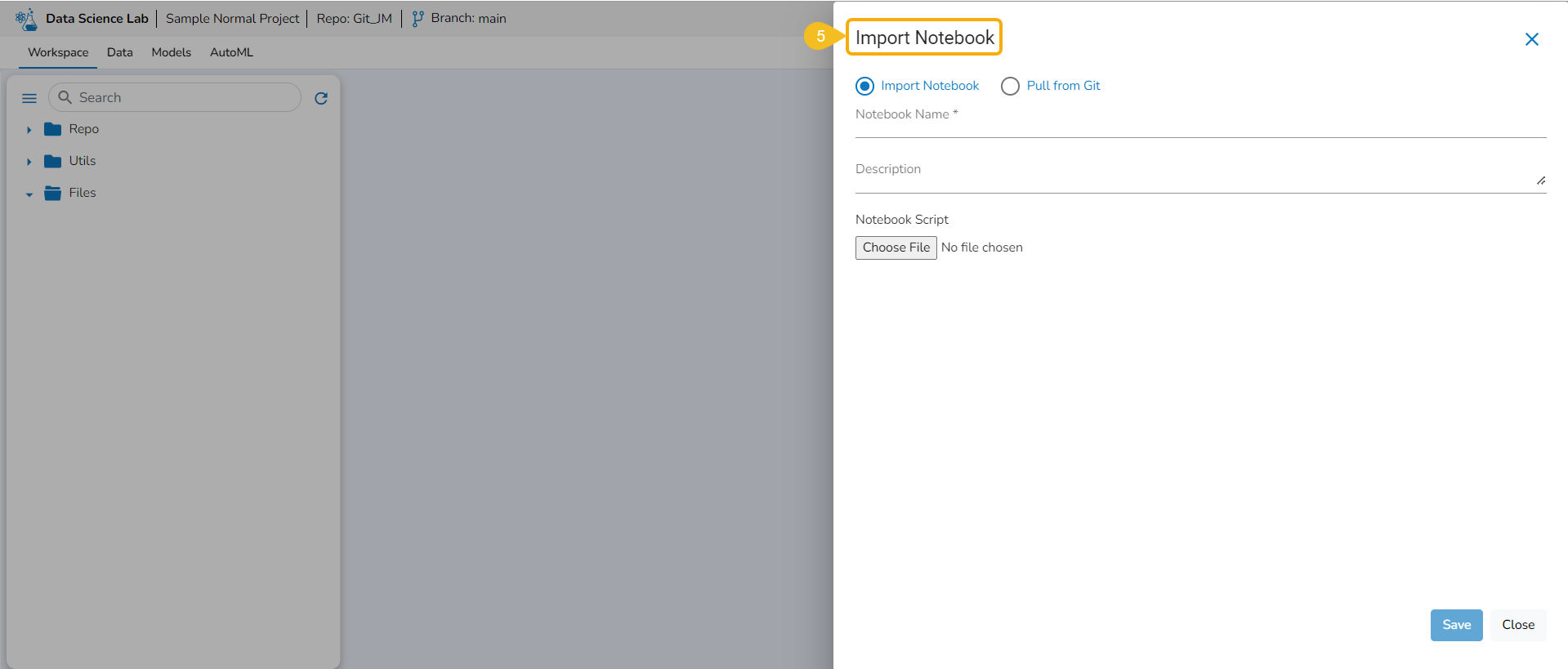
The Import Notebook page opens.
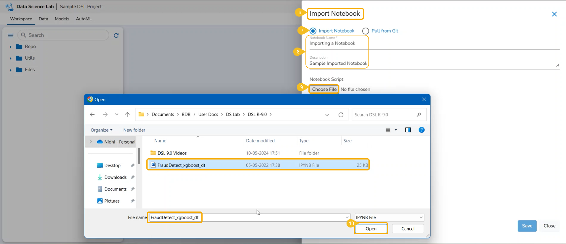
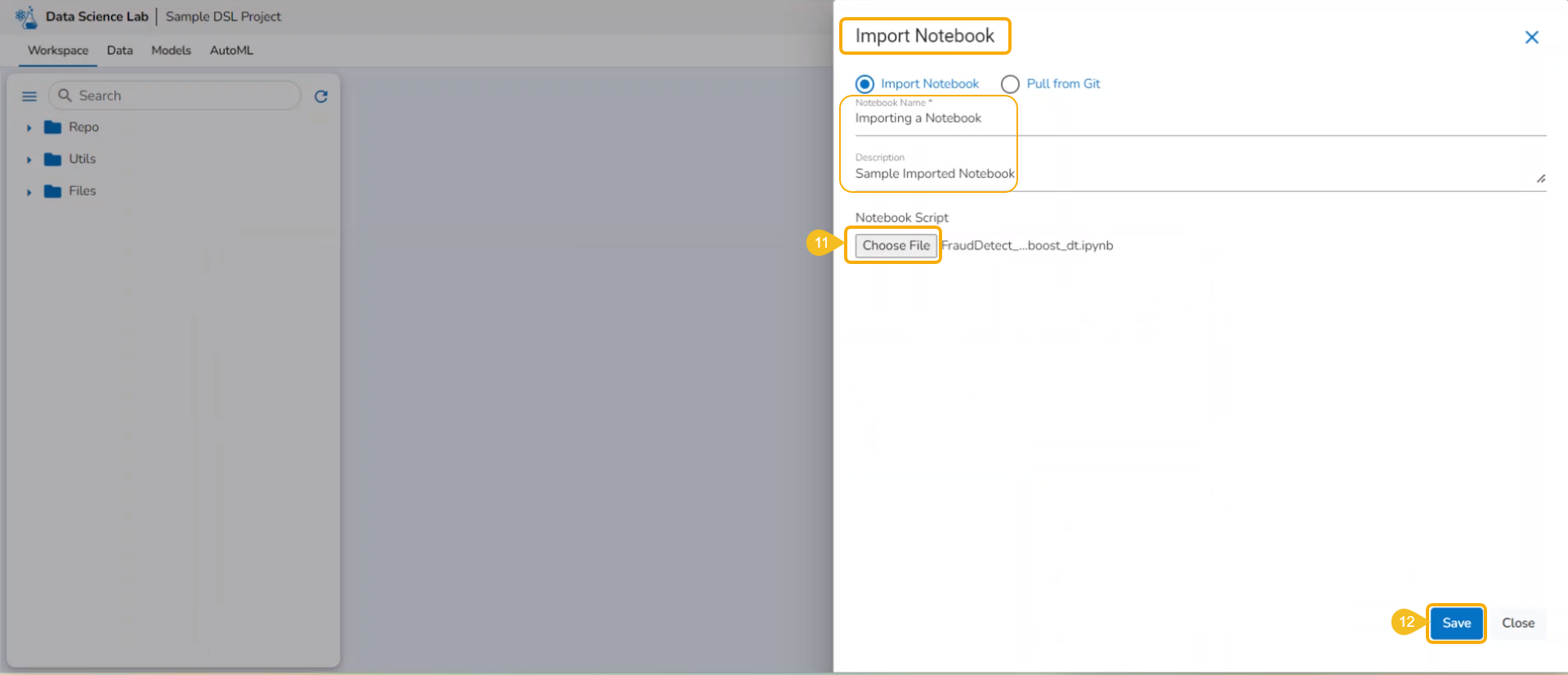
Select the Import Notebook option.
Provide the following information.
Notebook Name
Description (optional)
Click the Choose File option.
Select the IPYNB file from the system and upload it.
The selected file appears next to the Choose File option.
Click the Save option.
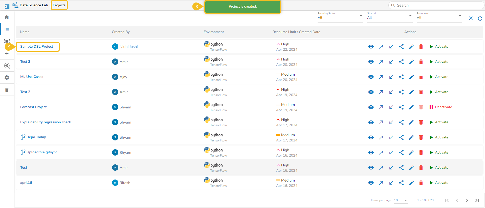
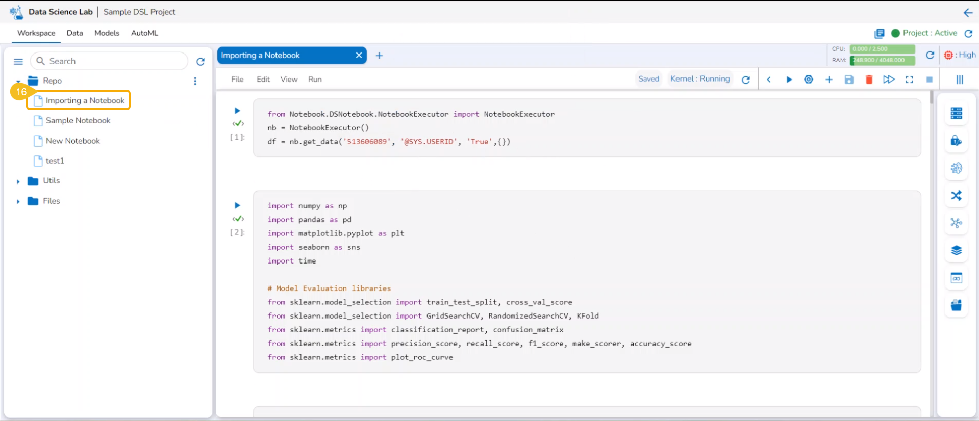
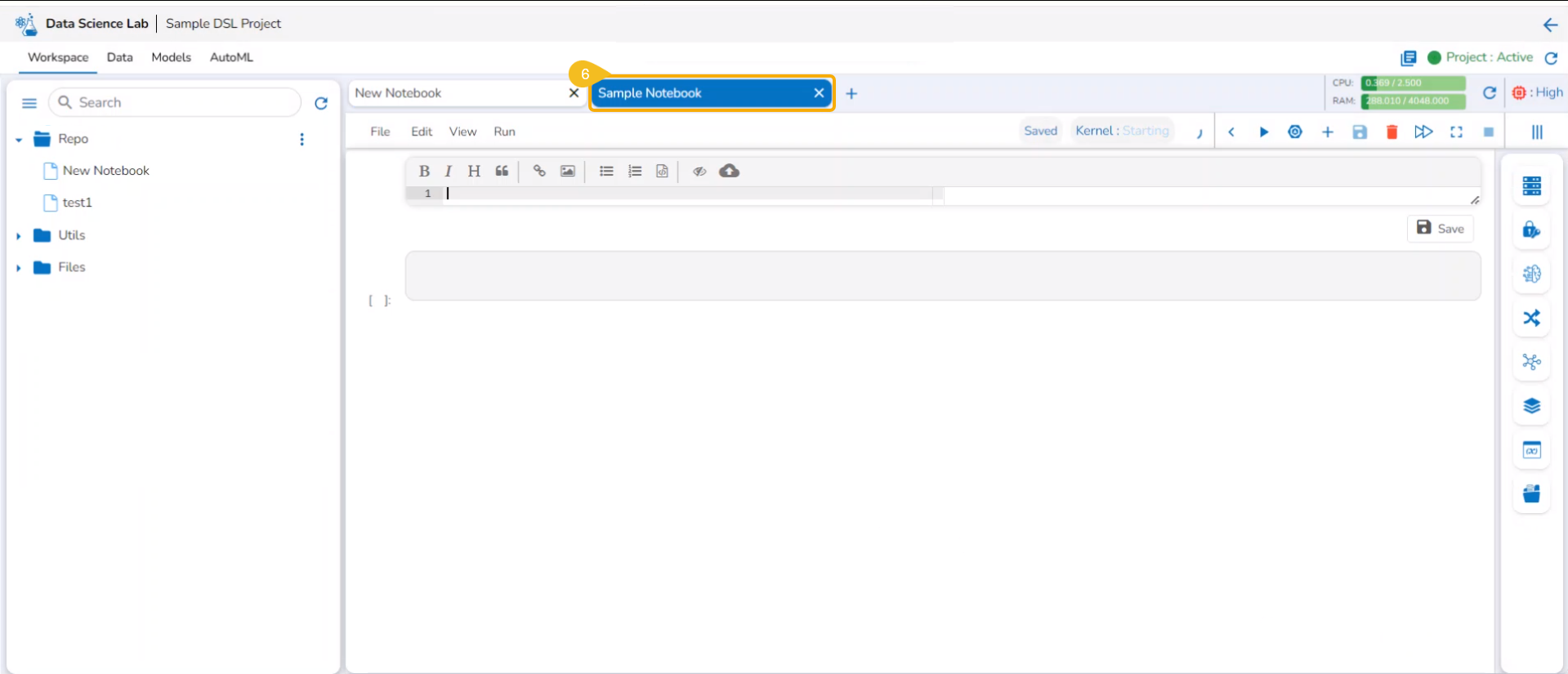
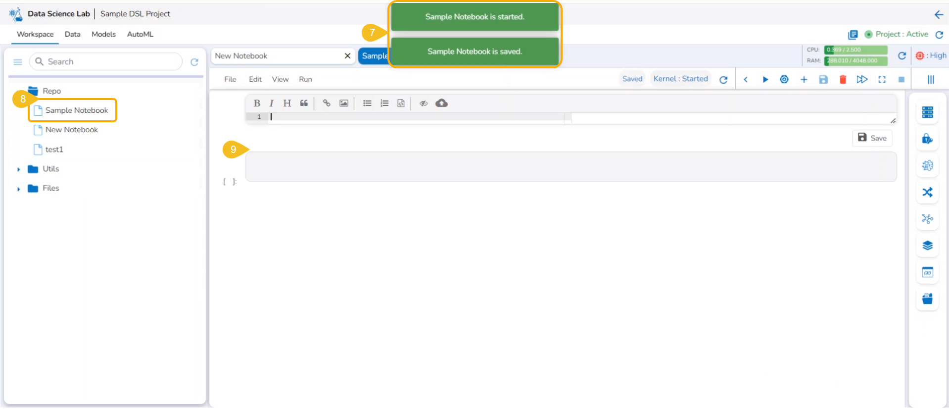
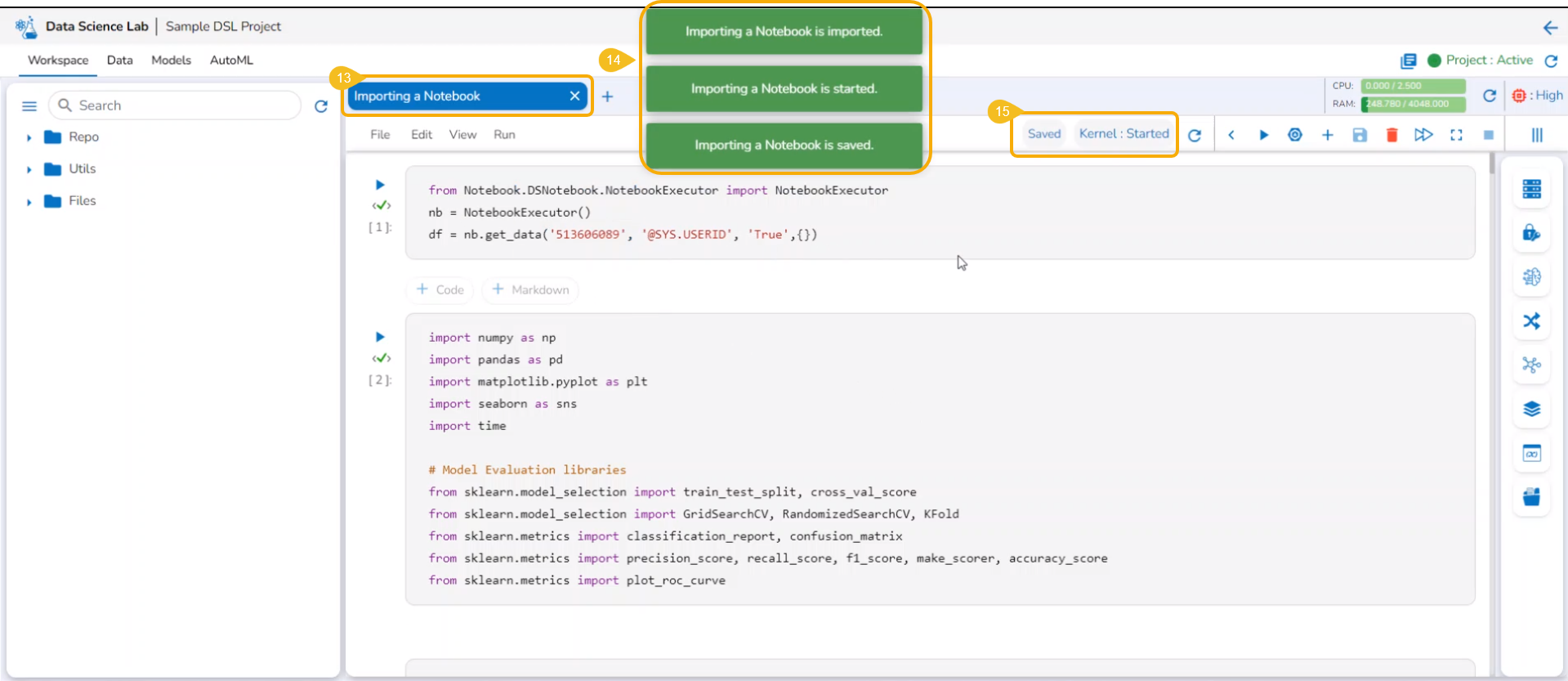
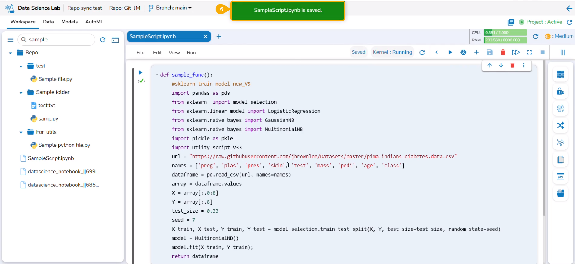
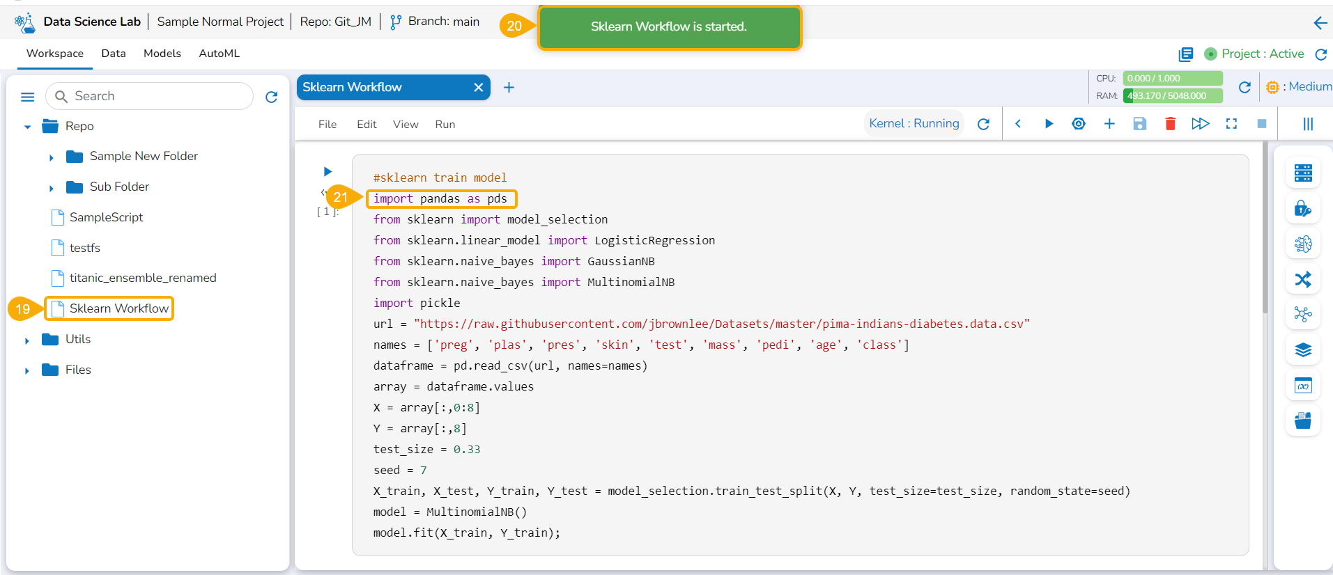
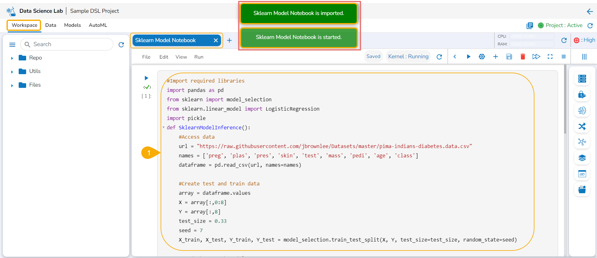
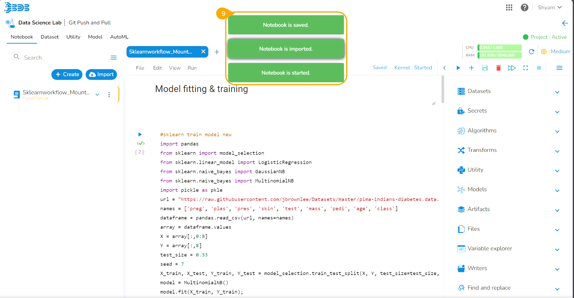
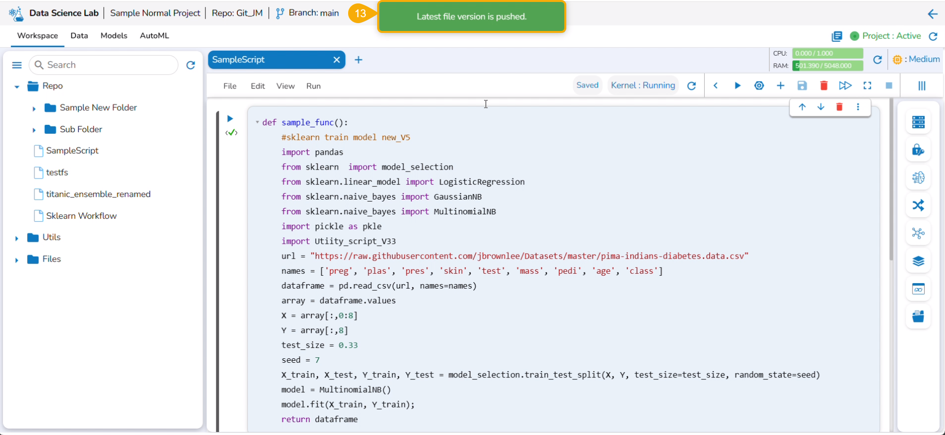
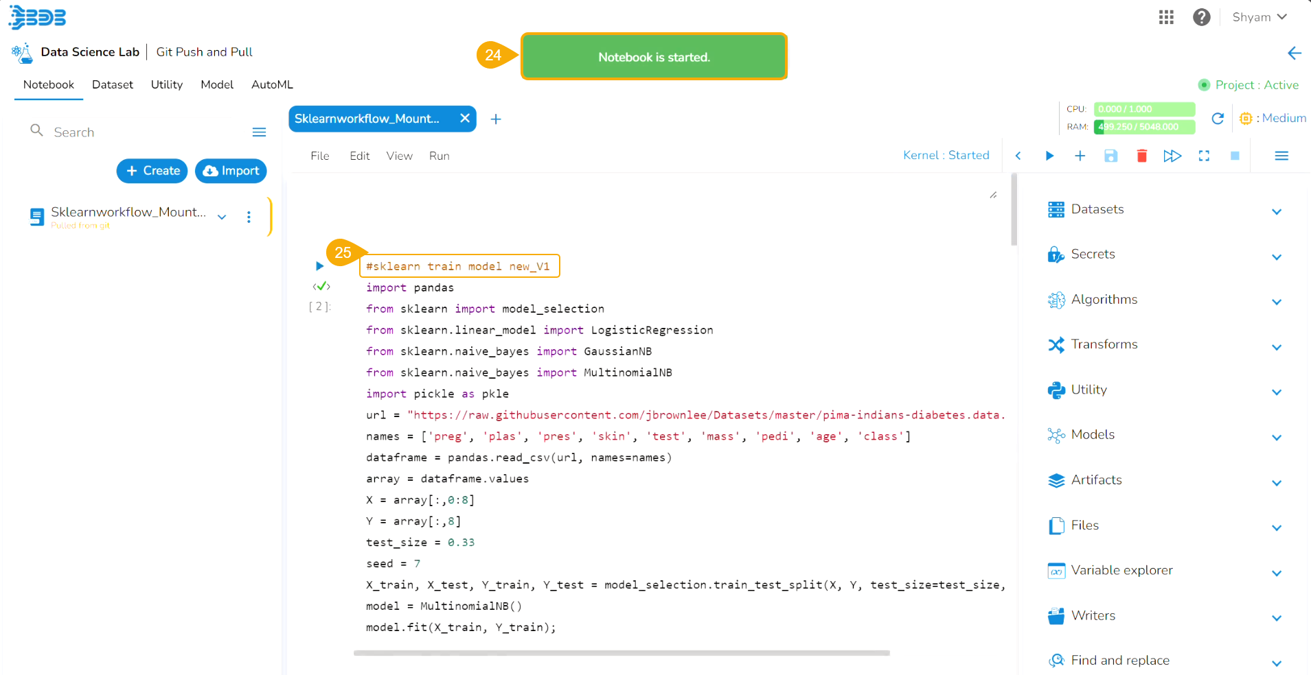
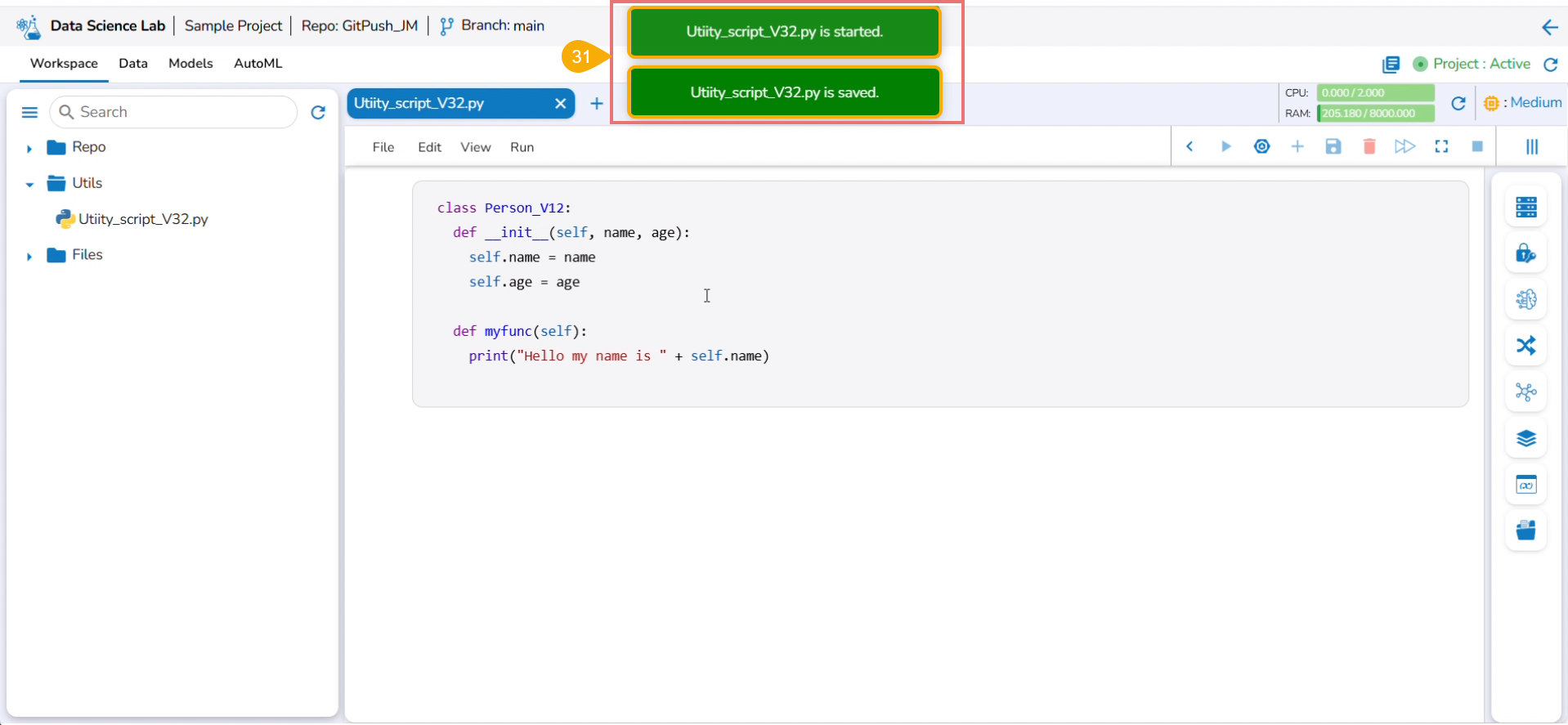
The Notebook infrastructure opens with the given name for the recently uploaded Notebook file. It may take a few seconds to save the uploaded Notebook and start Kernel for the same.
The following consecutive notification messages will appear to ensure the user that the Notebook is saved, uploaded, and started.
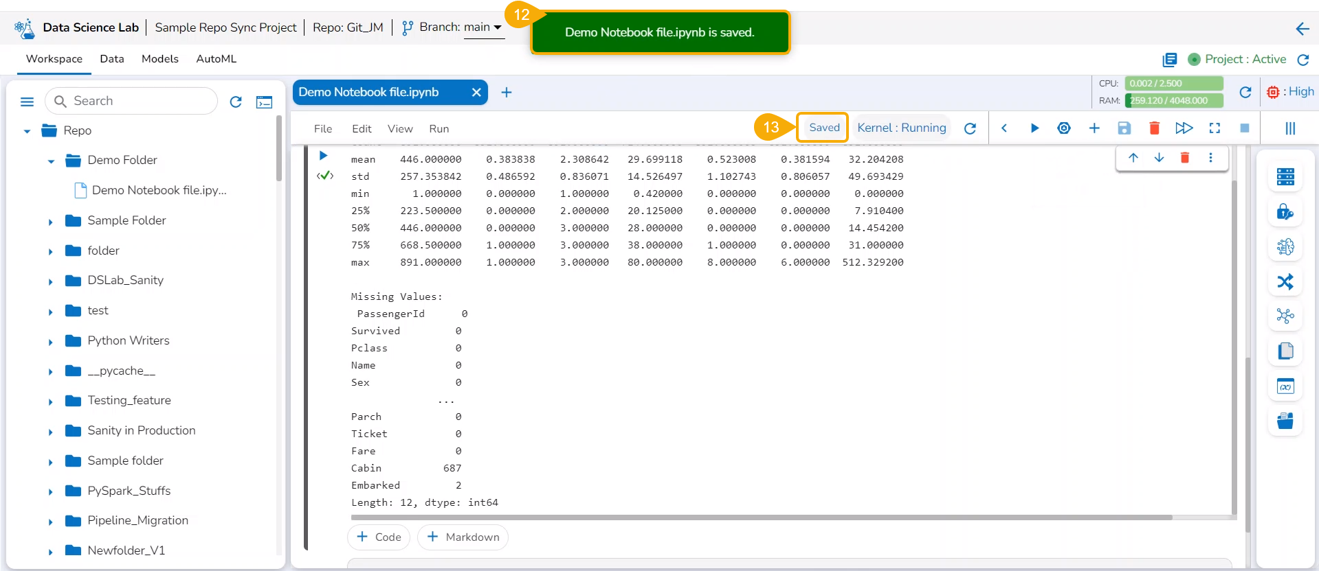
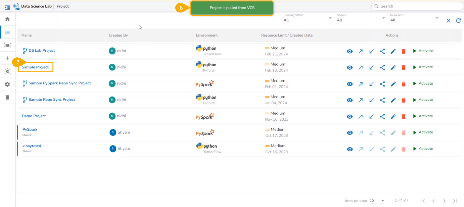
The same is mentioned by the status updates on the Notebook header (as highlighted in the given image).
The uploaded Notebook is listed on the left side of the page.
Please Note: The Imported Notebook will be credited with some actions. Refer to the Notebook Actions page to know it in detail.
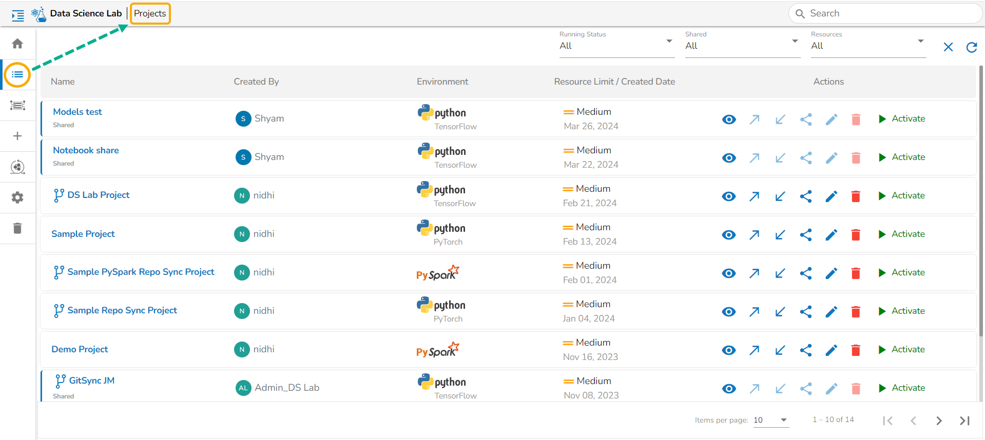
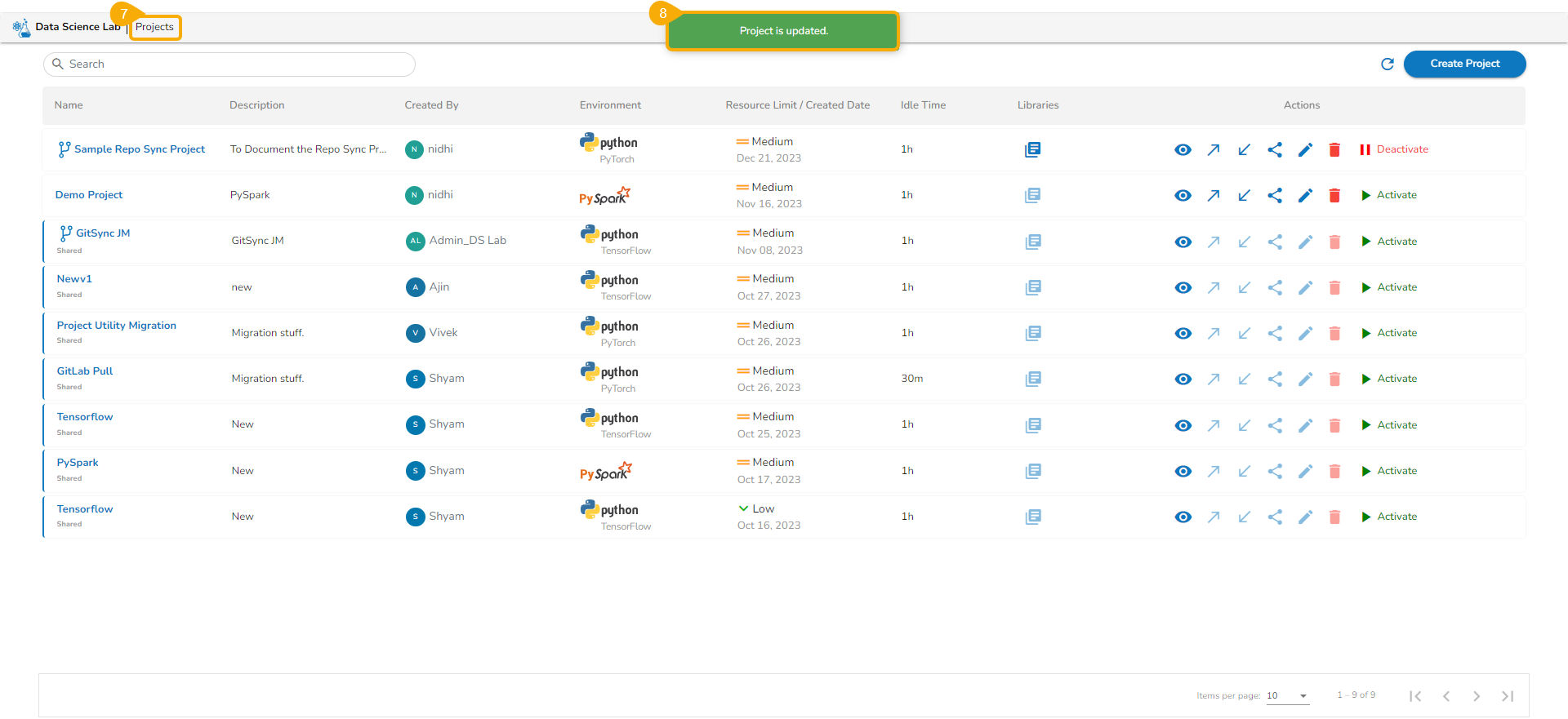
Projects
page.
Select a DSL project from the list.
Click the View icon.
The next page appears with the accessible tabs for the selected Project.
Tabs provided to a Python/TensorFlow DSL Project
If you select a PySpark project, the following tabs will be available:
Selecting a PySpark Project
Tabs provided for a PySpark Project
Various Tabs of a DSL Project
The following table provides an outlook of the various tabs provided to a DSL Project:
Name of the Tab
Functions covered by the tab
The Workspace tab inside a Repo Sync Project works like a placeholder to keep all the Git Hub & Git Lab Repository documents (folders and files) of the logged-in user.
The Data section focuses on how to add or upload data to your DSL Projects. This tab lists all the added Datasets, Data Stores, and Feature Stores for a Project.
The Model tab includes various models created, saved, or imported using the Data Science Lab module. It broadly lists Data Science Models, Imported Models, and Auto ML models.
Please Note: The allocation of tabs to a DSL project is environment-based.
If the user selects the PySpark environment, the available tabs to the user will be Workspace and Data. The user will not have access to the Models and AutoML tabs.
The DSL Projects created based on PythonTensorFlow and Python PyTorch environments will contain all four tabs.
Import
options under the
Workspace
landing page.
Accessing the Workspace Tab for a Repo Sync Projects
Navigate to the Projects page.
Select an activated Repo Sync Project from the displayed list.
Click the View icon to open the project.
The Repo Sync project opens displaying the Workspace tab.
A Repo folder gets added to the selected Repo Sync project based on the selected Git repository account (at the user-level settings) under the Notebook tab with Refresh and Git Console icons.
Icons
Name of the Icons
Actions
Refresh
Refreshes the data taken from the selected Git Repository.
Git Console
Opens a console page to use Git Commands.
Please Note:
The Repo Sync Project opens with a branch configured at the project level.
A Repo Sync Project contains other than .ipynb files under the Workspace tab.
Accessing the Workspace Tab for other Data Science Projects
Navigate to the Projects page.
Select an activated Project from the displayed list.
Click the View icon to open the project.
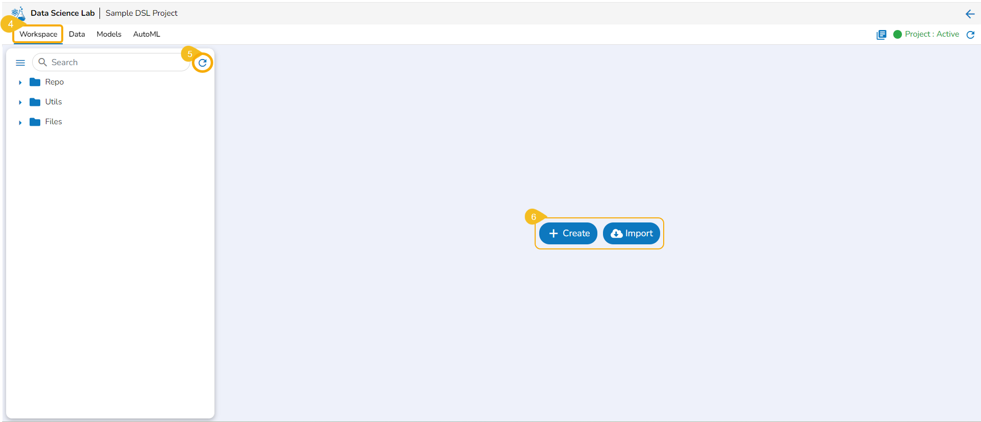
The Project opens displaying the Workspace tab.
The Repo, Utils, and Files default folders appear under the Workspace tab.
Please Note: If the selected project is a Repo Sync Project, it will only contain a Repo folder under the Workspace tab. Here, the Repo folder will support all file types. Three folders (Repo, Utils, and Files) will be available under the Workspace tab for a normal Data Science Lab project.
A Refresh icon is provided to refresh the data.
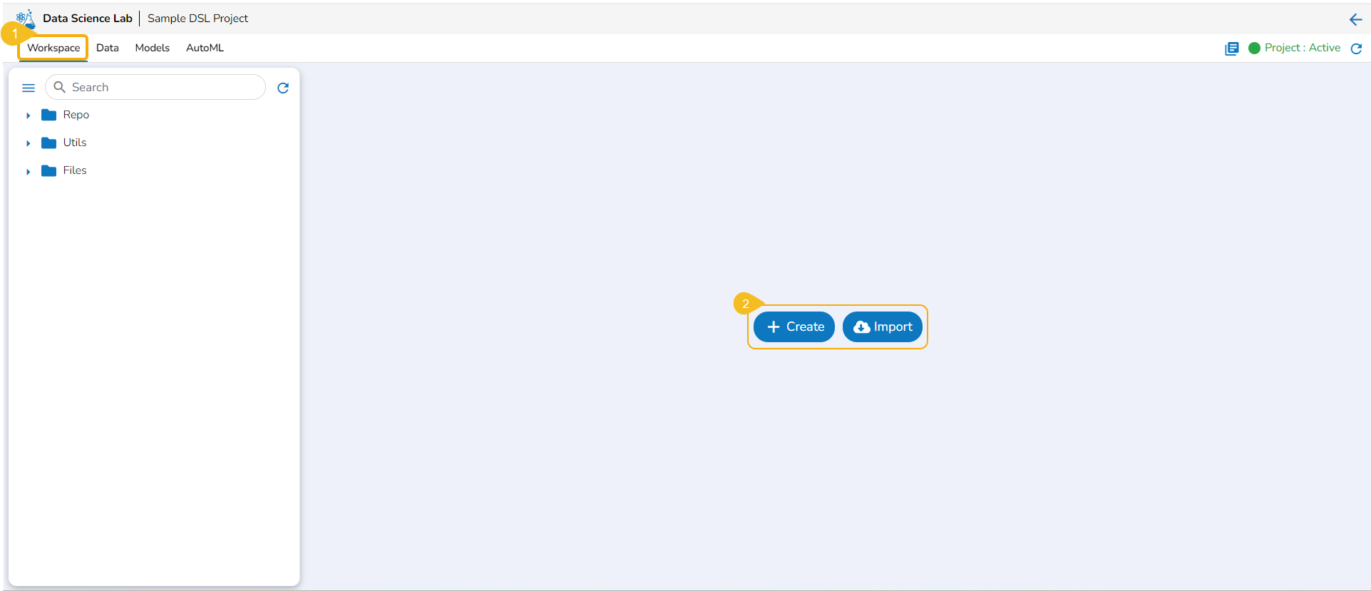
The users get two options to start with their data science exploration:
Create - By Creating a new Notebook
Import -By Importing a Notebook
Libraries
The Libraries icon on the Workspace displays all the installed libraries with version and status.
Navigate to the Workspace tab.
Click the Libraries icon.
The Libraries window opens displaying Versions and Status for all the installed libraries.
Click the Failed status to expand the details of a failed library installation.
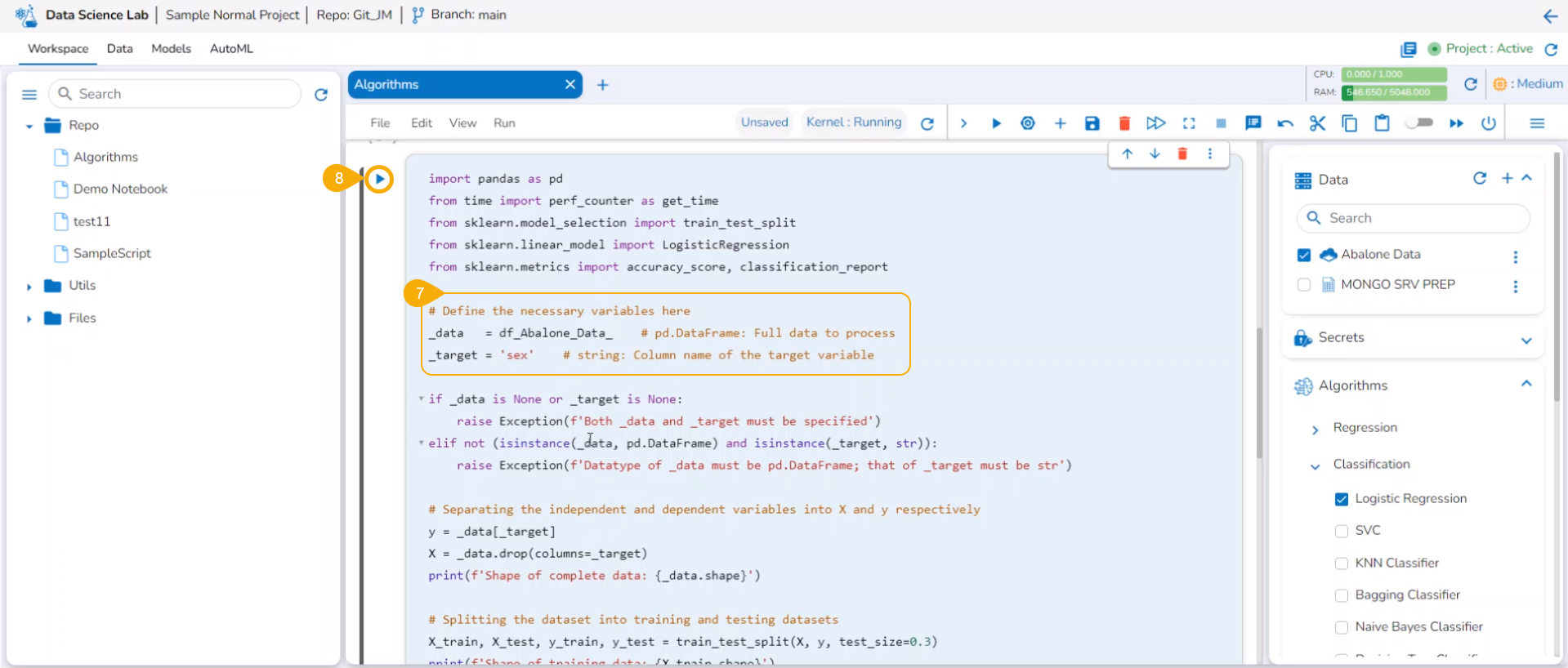
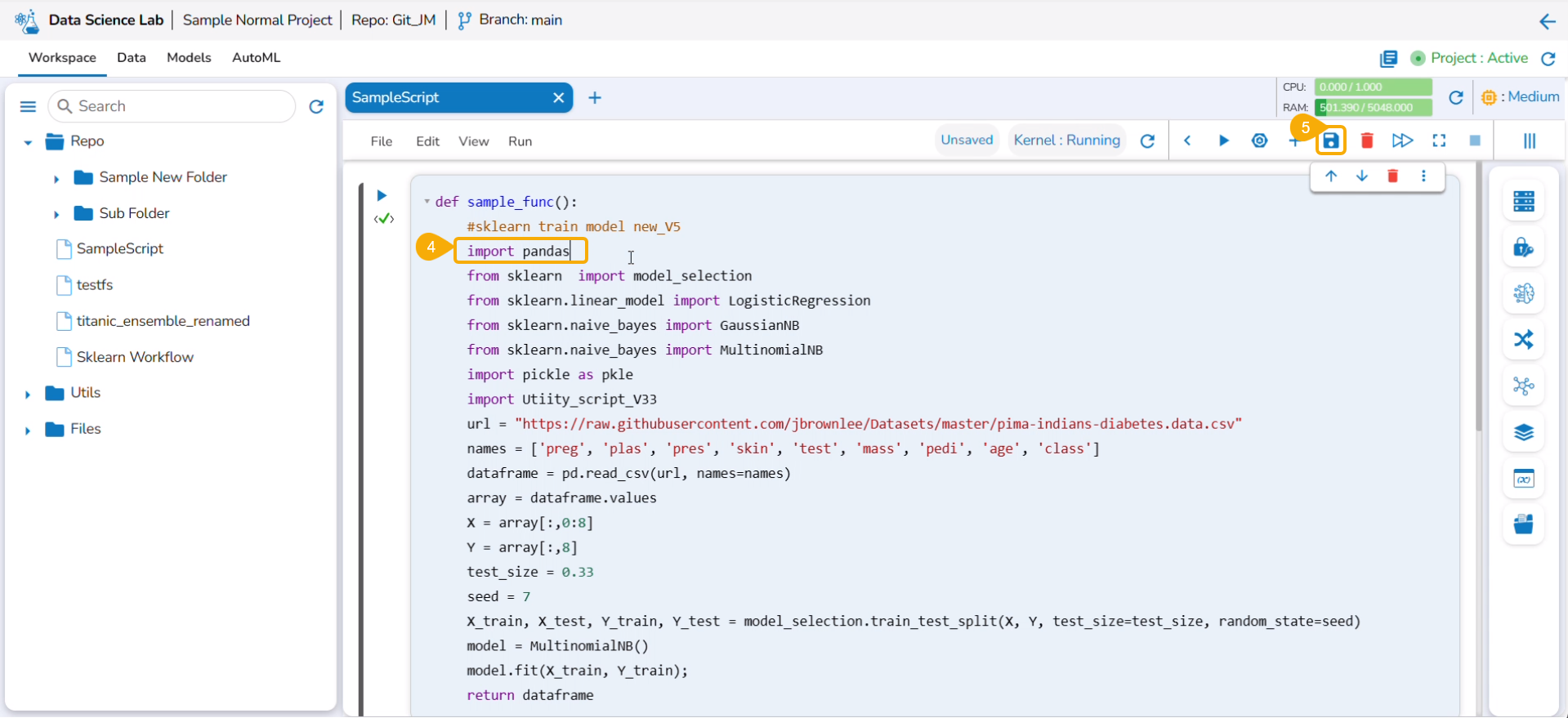
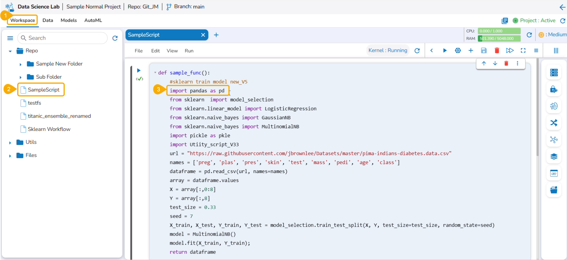
Saving a Data Science Lab Model
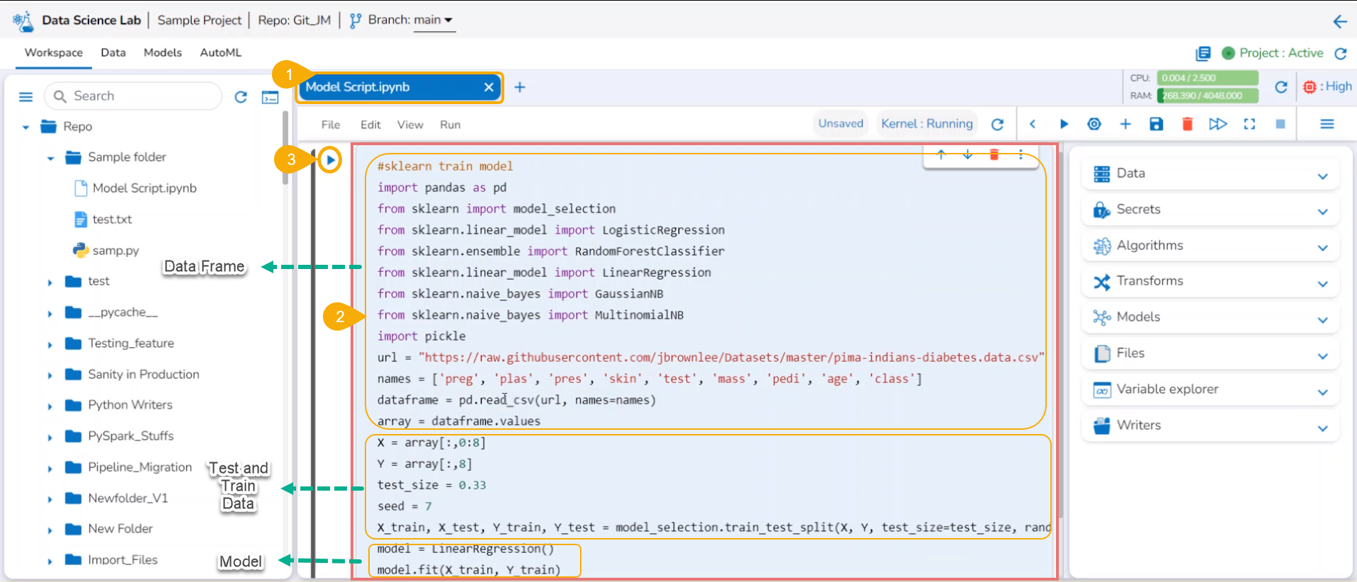
Navigate to a Data Science Notebook.
Write code using the following sequence:
Read DataFrame
Define test and train data
Create a model
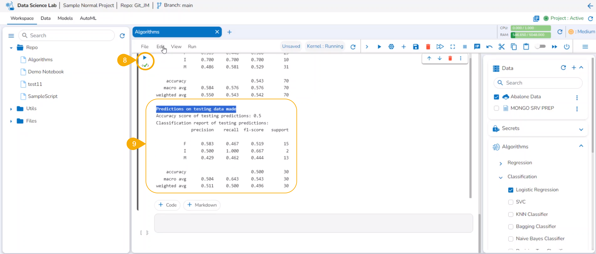
Execute the script by running the code cell.
Sample Script for a Data Science Model
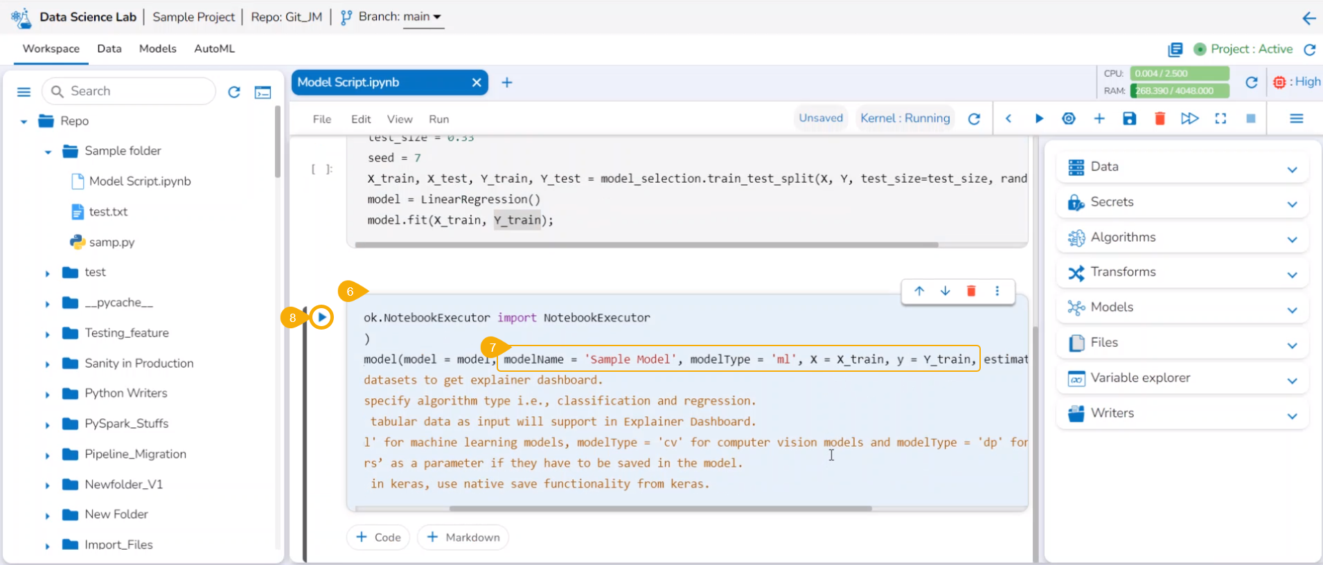
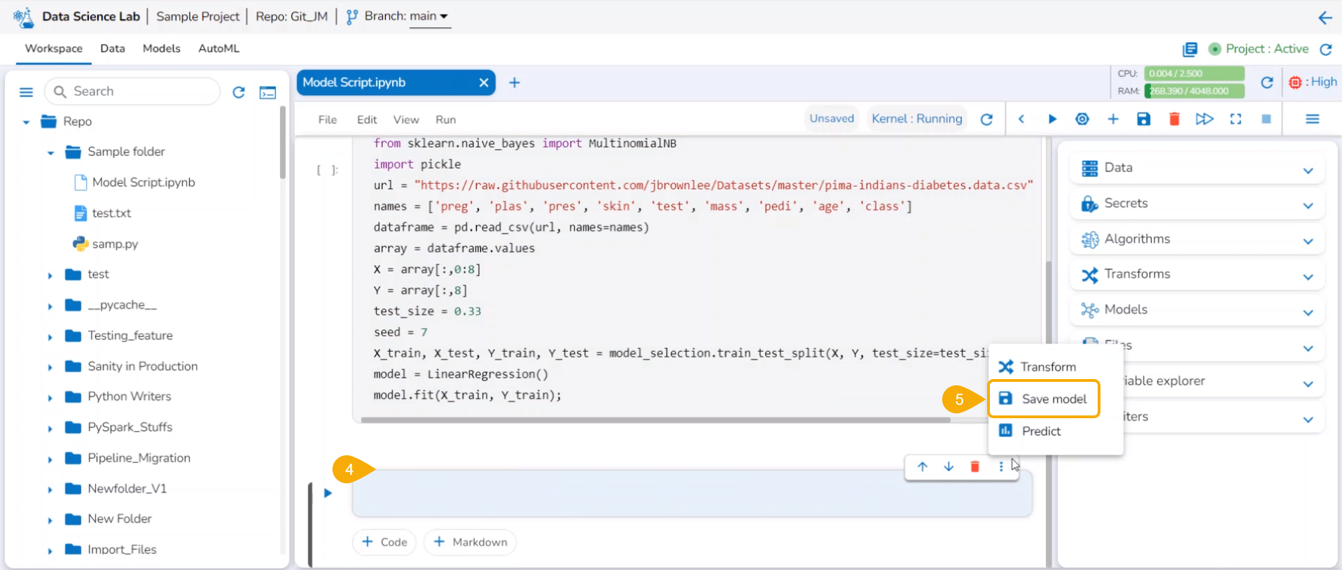
Get a new cell.
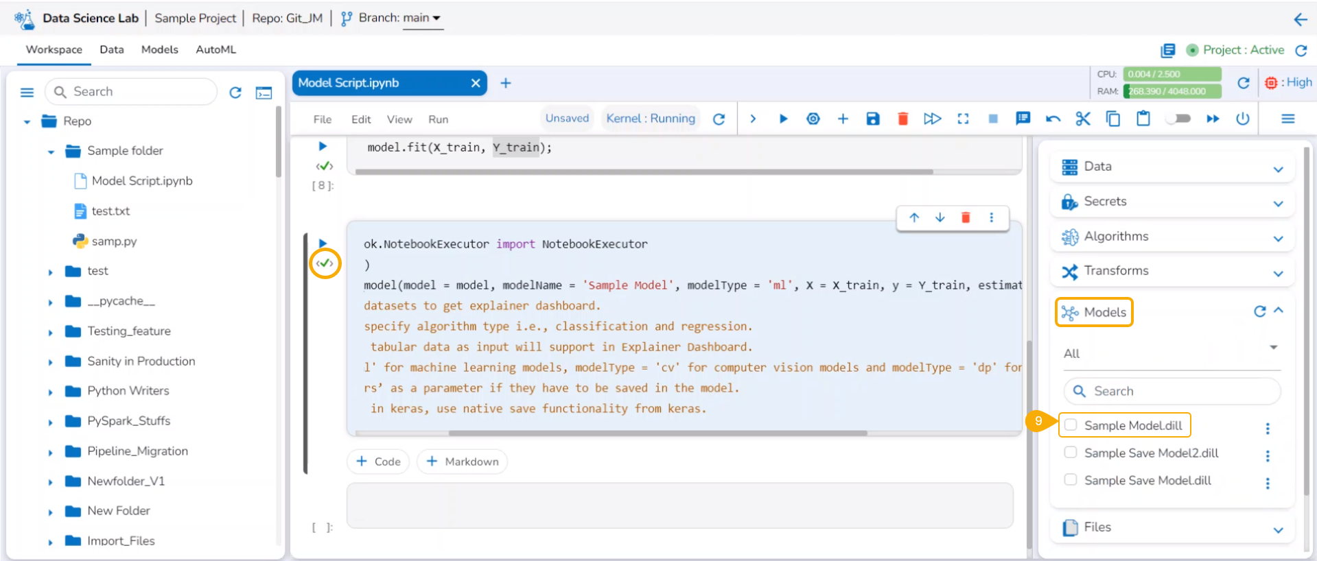
Click the Save model option.
A code gets generated in the newly added code cell.
Give a model name to specify the model and model type as ml.
Execute the code cell.
After the code gets executed, the Model gets saved under the Models tab.
the model gets saved
Please Note: The newly saved model gets saved under the unregistered category inside the Models tab.
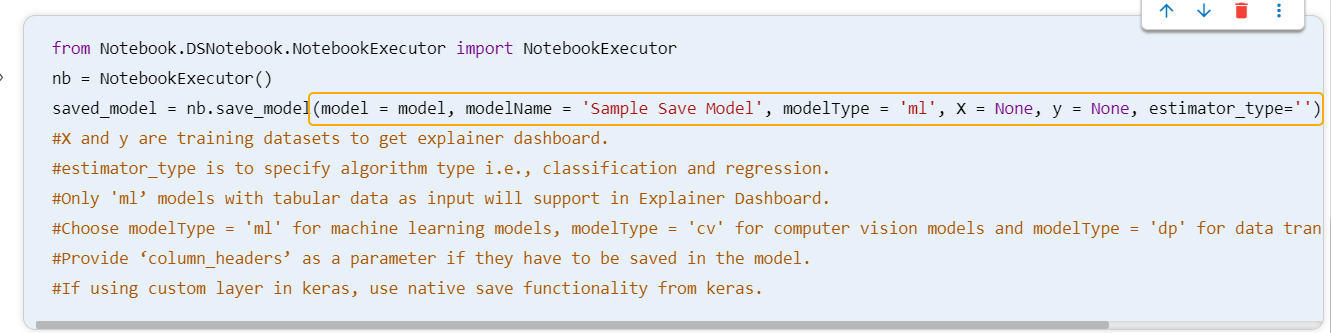
Function Parameters
model - Trained model variable name.
modelName - The desired name given by the user for the trained model.
modelType - Type in which model can be saved.
X - This array contains the input features or predictors used to train the model. Each row in the X_train array represents a sample or observation in the training set, and each column represents a feature or variable.
Y - This array contains the corresponding output or response variable for each sample in the training set. It is also called the target variable, dependent variable, or label. The Y_train array has the same number of rows as the X_train array.
estimator_type - The estimator_type of a data science model refers to the type of estimator used.
Specify a Data Science Lab Model by giving a Model name & Model Type
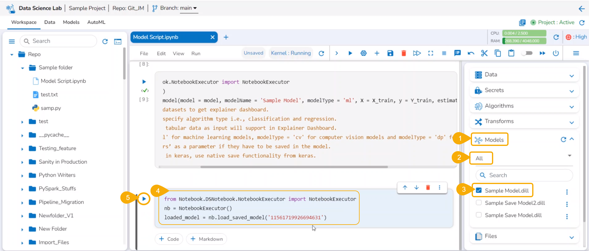
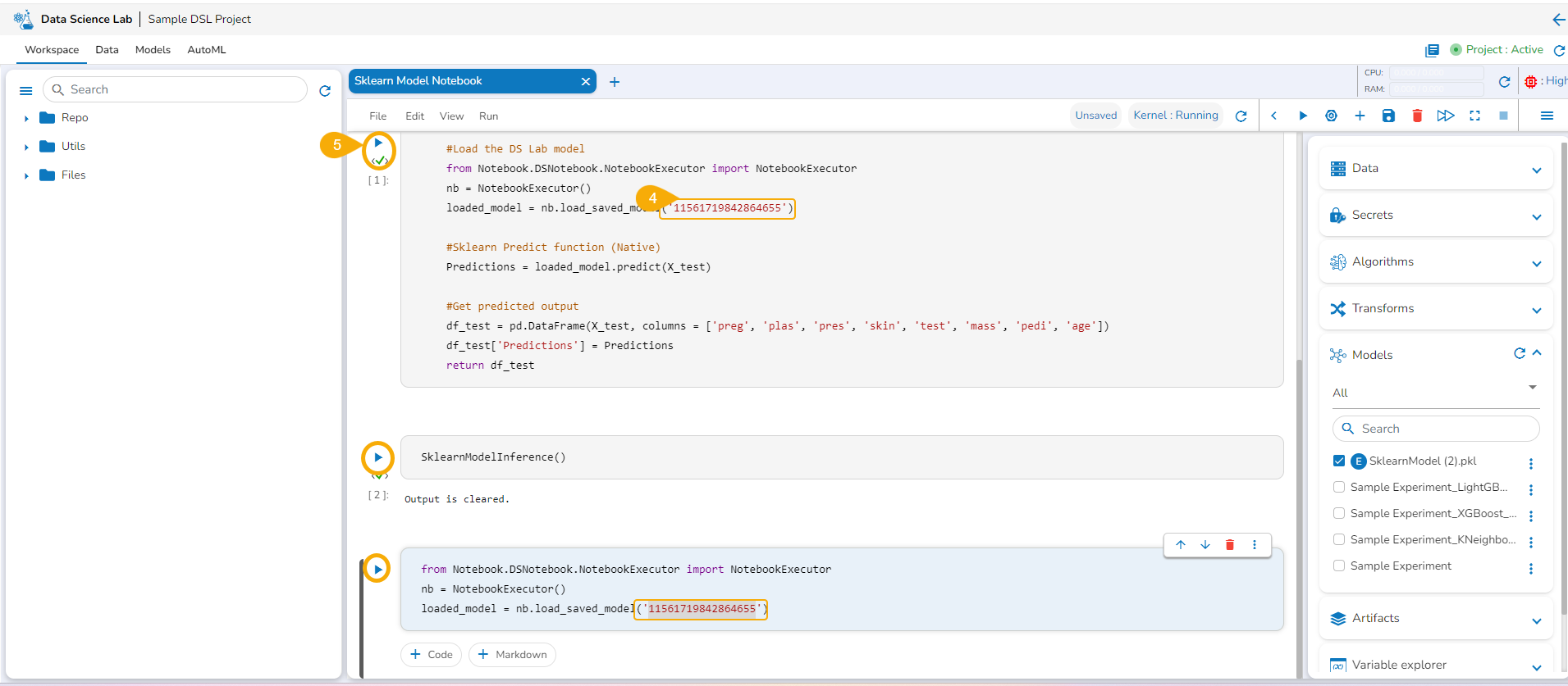
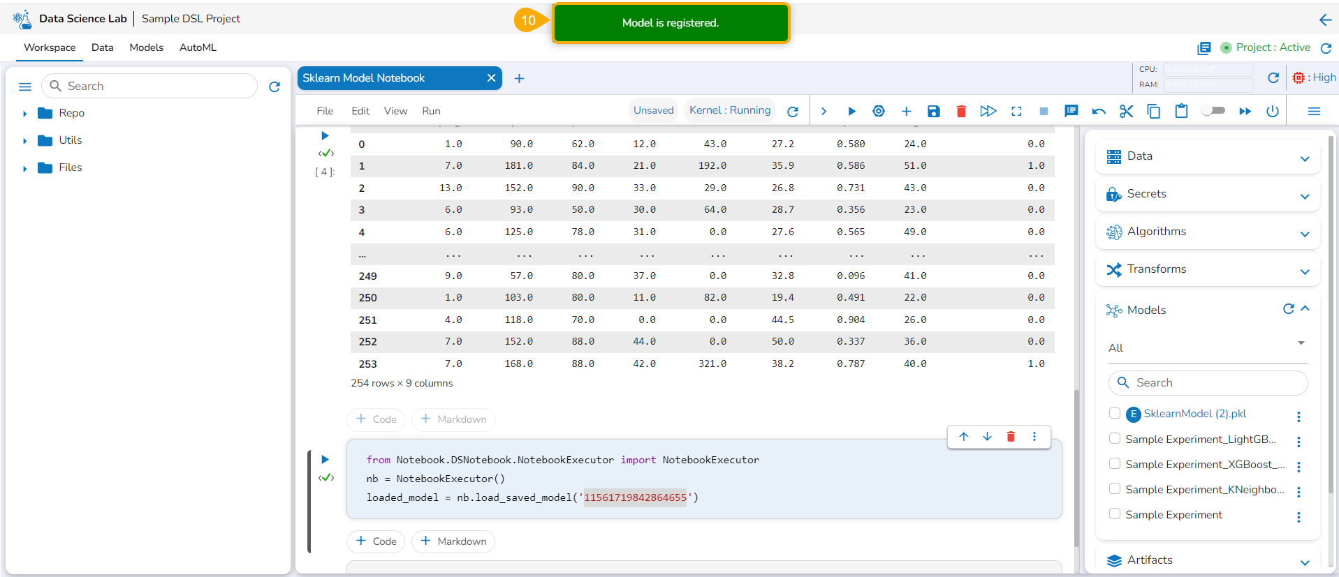
Loading a Data Science Lab Model
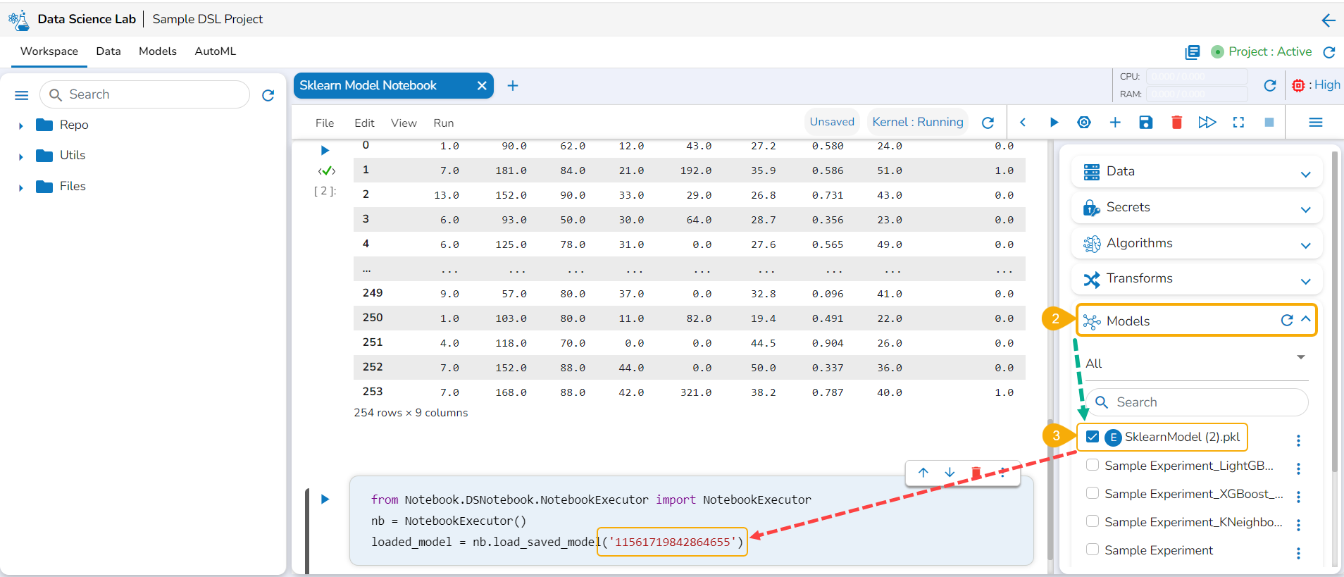
Open the Models tab.
Access the Unregistered category.
The savedmodel will be available under the Models tab. Please select the model by using the given checkbox to load it.
The model gets loaded into a new cell.
Run the cell.
Loading a saved Data Science Lab Model
Navigate to a Data Science Notebook.
Add a new cell.
Provide Data set.
Define DataFrame and execute the cell.
A new cell will be added below.
Click the Ellipsis icon to access more options.
Select the Save Artifacts option.
Give proper DataFrame name and Name of Artifacts (with extensions - .csv/.txt/.json)
Execute the cell.
The Artifacts get saved under the Artifacts tab.
Please Note:
The saved Artifacts can be downloaded as well.
The user can also get an instant visual depiction of the data based on their executed scripts.
Preview Artifacts
Navigate to the Artifacts tab inside a DS Notebook page.
Select a saved Artifact from the right side panel.
Click the vertical ellipsis icon for the saved Artifact.
Click the Preview option from the context menu.
The Artifact Preview gets displayed.
Please Note:
The selected Artifact gets deleted from the list by clicking the Delete option.
Open the Variable Explorer tab.
The variables will be listed below under the Name column.
By hovering the cursor on a variable, you can get a mention of the name, type, and shape details of the selected variable.
Click the Explore icon.
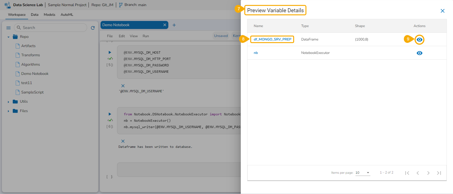
The Preview Variable Details page opens.
Select a Variable from the displayed list.
Click the Preview icon provided for the selected Variable.
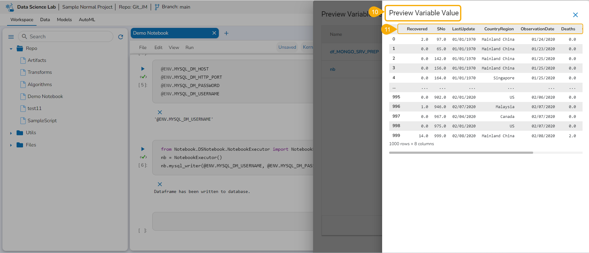
The Preview Variable Value page opens.
All the values of the selected Variable are displayed in a tabular format.
Accessing the Unregister option from the Model list
Confirmation message after the model gets unregistered
Listing unregistered Model under the Model tab
Information option for a Notebook
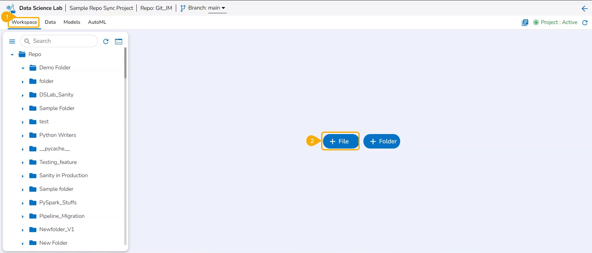
Adding File and Folders
These options are provided under the Workspace tab of a repo sync folder.
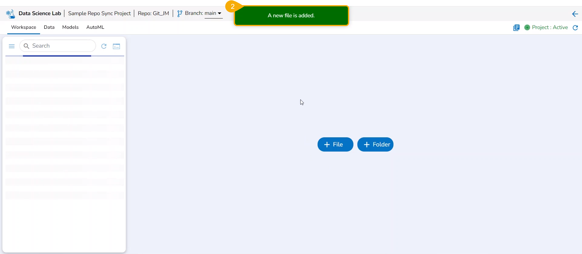
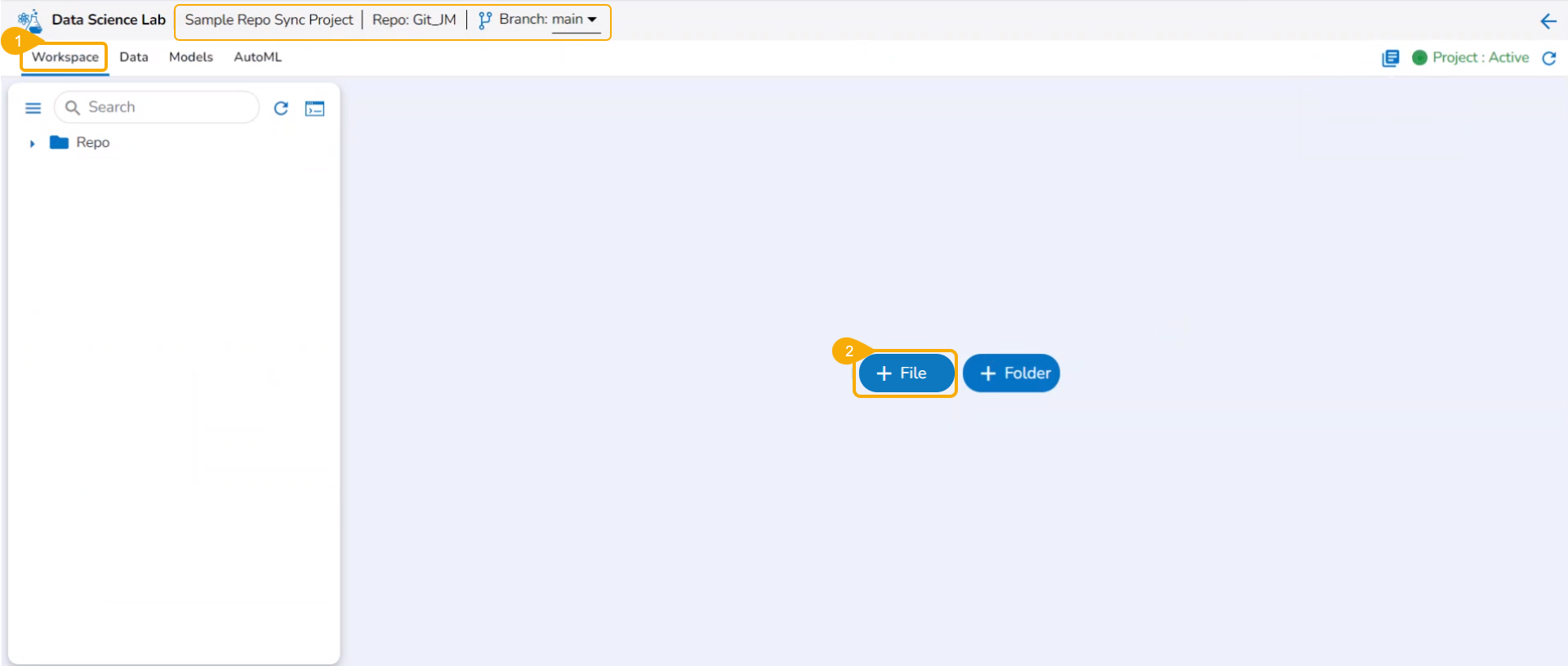
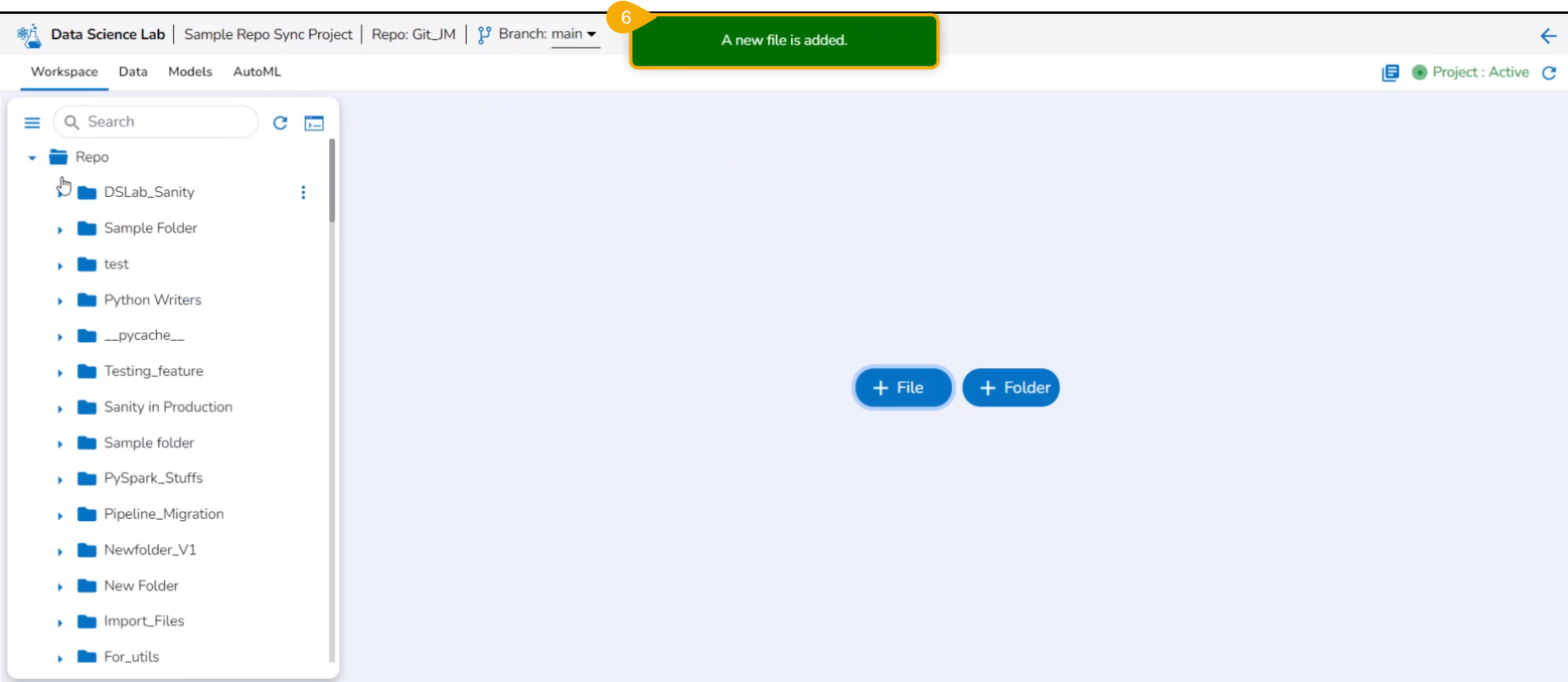
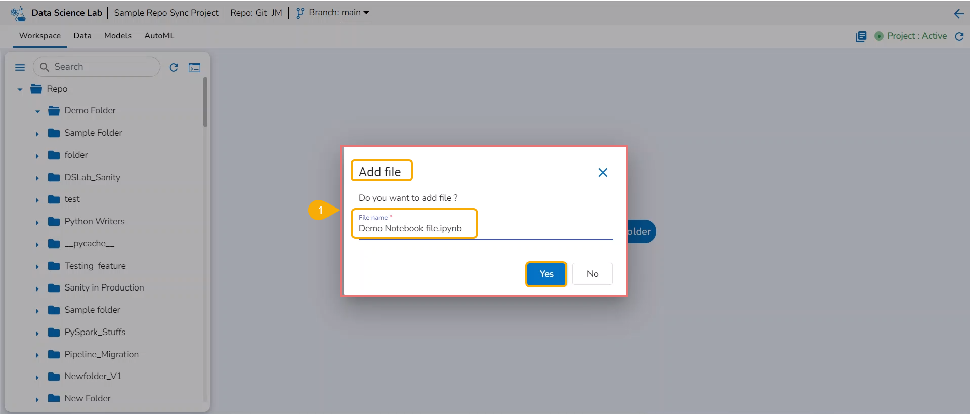
Adding a File
Check out the illustration on how to add a file inside a Repo Sync Project.
Navigate to the Workspace tab of an activated Repo SyncProject.
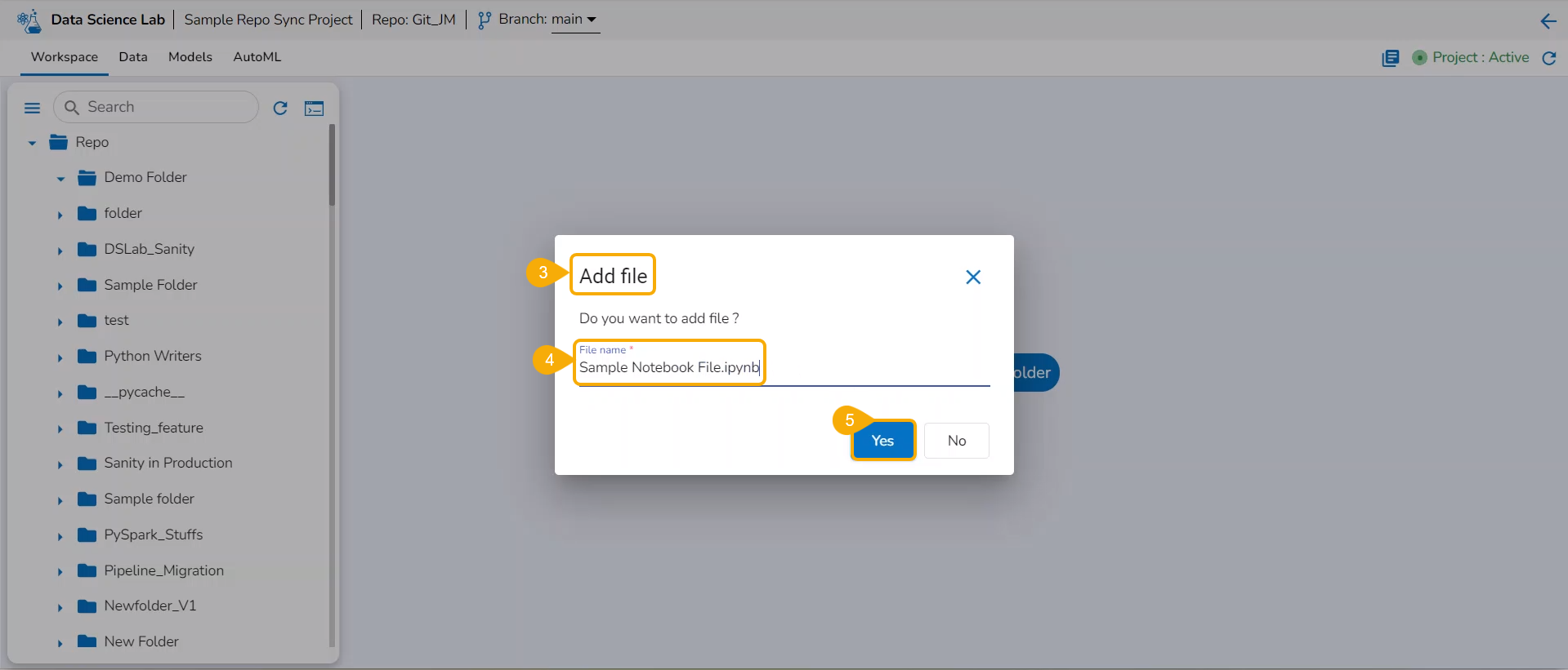
Click the Add File option.
The Add file window opens.
Provide a File name.
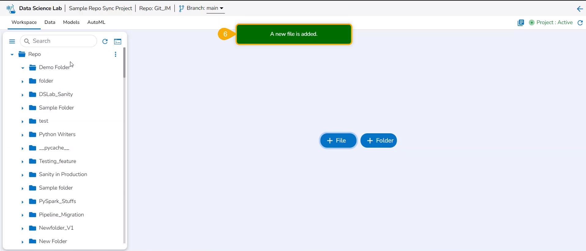
Click the Yes option.
A notification message appears to ensure that the new file has been created.
The newly created file gets added to the Repo Sync Project.
Defining a File Type
The user can insert the file type while adding a file to define the file type.
Check out the illustration on defining a file type while adding a file to the Repo Sync project.
Navigate to the Workspace tab for a repo sync project.
Click the Add File option.
The Add file window opens.
File name: Provide the file type extension while giving it a name.
Click the Yes option.
A notification message appears.
The new file gets added with the provided file extension.
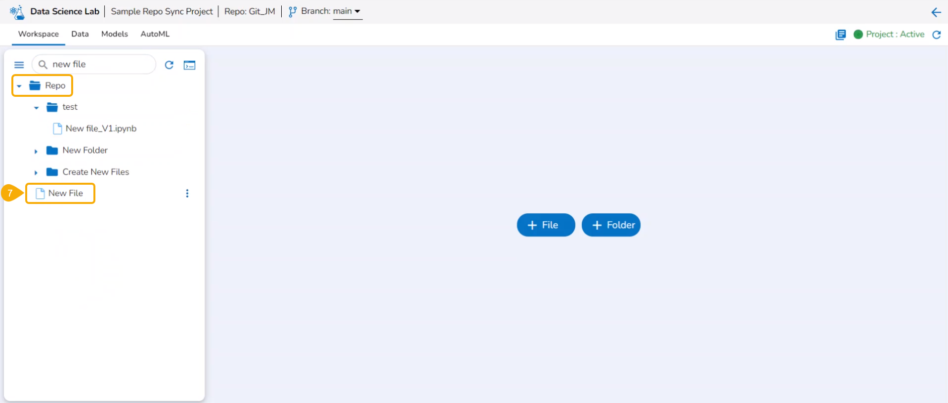
Adding a New Folder
Check out the illustration on how to add a folder inside a Repo Sync Project.
Navigate to the Notebook tab of the Repo Sync Project.
Click the Add Folder option.
The Add folder window opens.
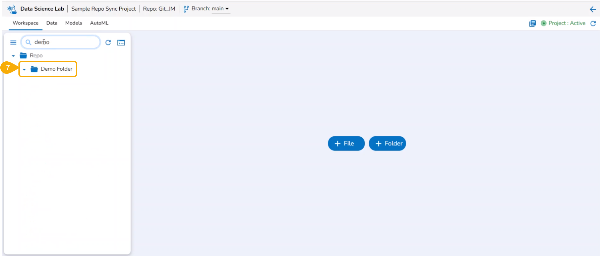
Provide a Folder name.
Click the Yes option.
A notification message appears to ensure that the new folder has been created.
The newly created folder gets added to the Repo folder.
Creating AutoML Experiment
A Data Scientist can create various Experiments based on specified algorithms.
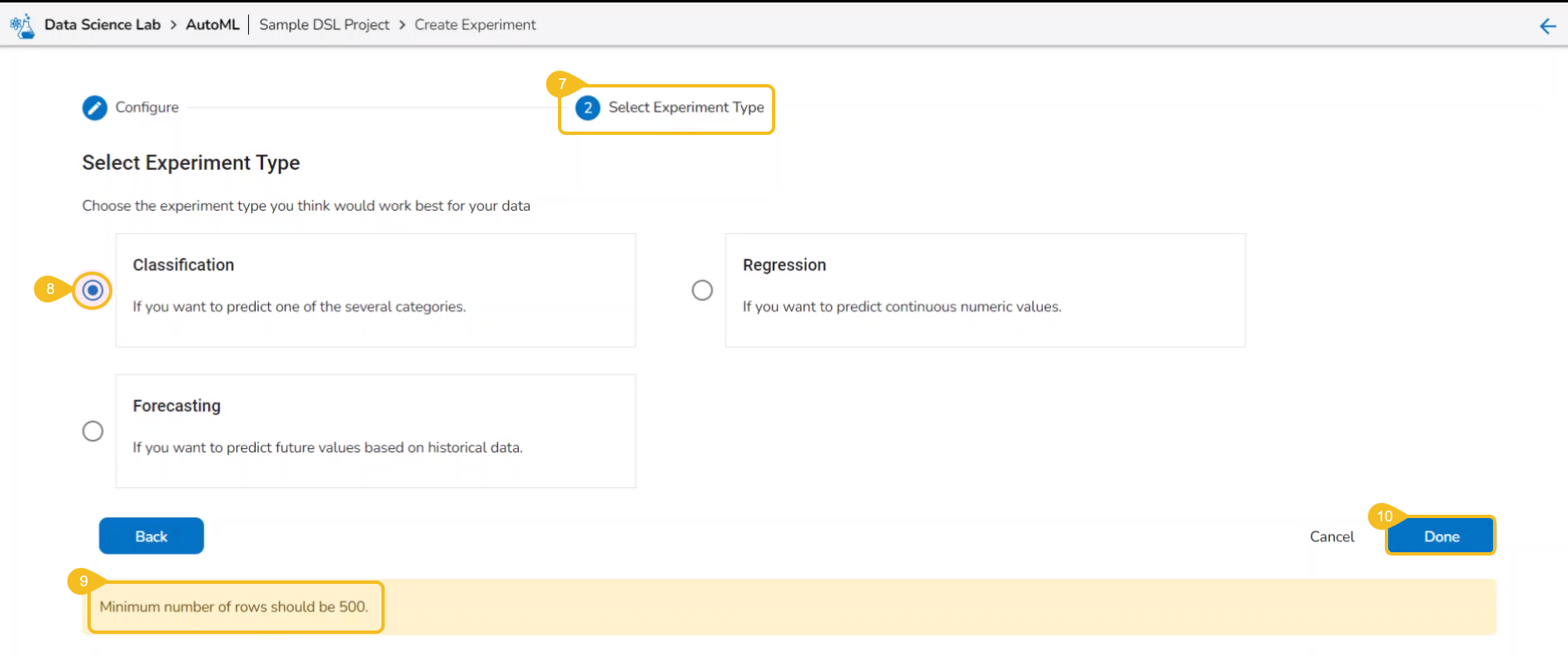
There can be different types of Experiments based on the algorithm type specified. In the DS Lab module, we currently support Classification, Regression, and Forecasting.
A Classification experiment can be created for discrete data when the user wants to predict one of the several categories.
A Regression experiment can be created for continuous numeric values.
A Forecasting experiment can be created to predict future values based on historical data.
Please Note:
AutoML experiments are running as Jobs, and a new Job will be allocated for each experiment created in the AutoML tab.
Jobs will spin up once the Experiment is created, and after models are trained and ready, it will get killed automatically.
Creating an AutoML Experiment
Creating an Experiment is a two-step process that involves configuration and selection of the algorithm type as steps.
A user can create a supervised learning (data science) experiment by choosing the Create Experiment option.
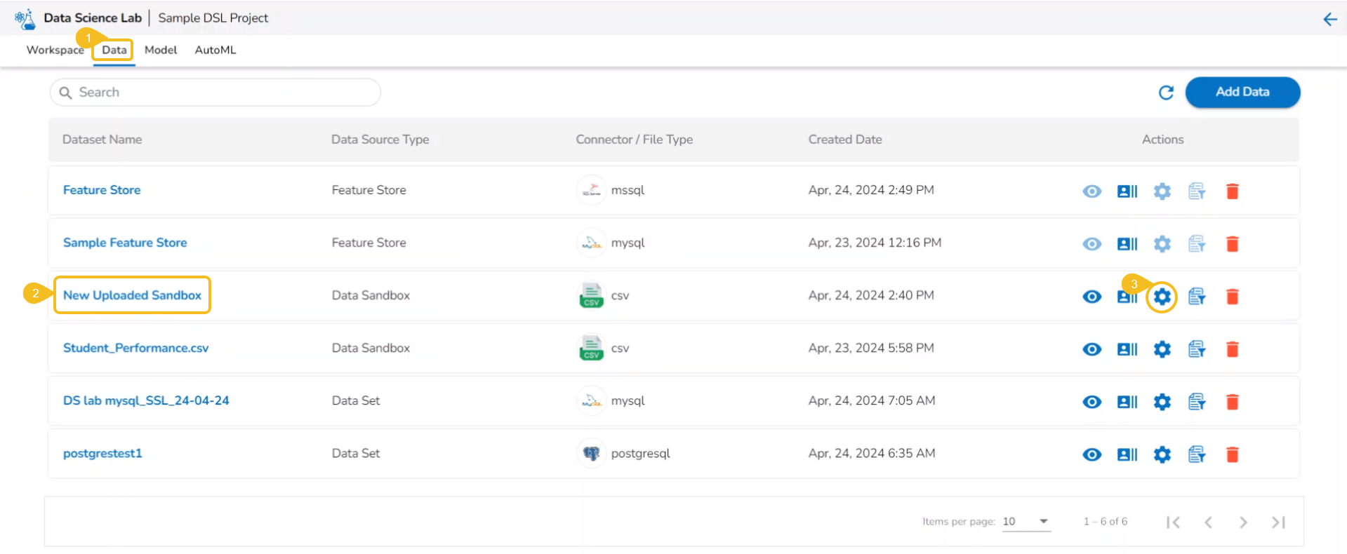
Please Note: The Create Experiment icon is provided on the Dataset List page under the Dataset tab of a Repo Sync Data Science Project.
Navigate to the Data List page.
Select a Dataset from the list.
Click the Create Experiment icon.
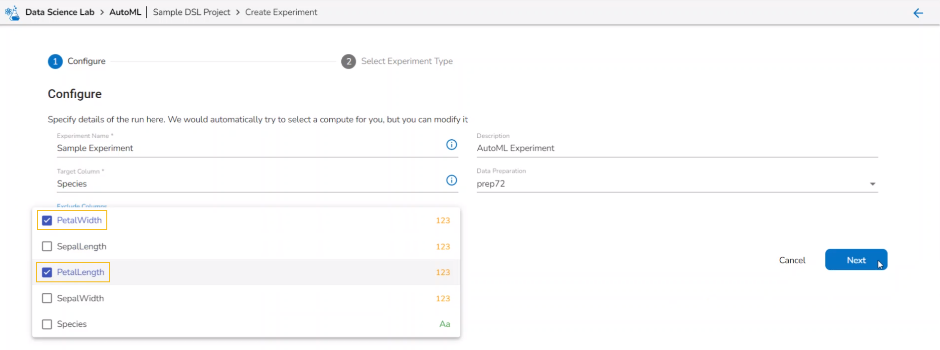
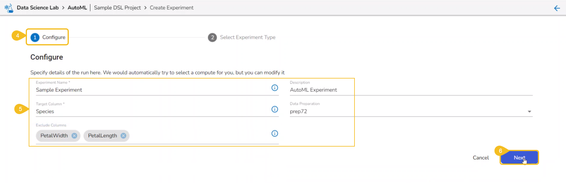
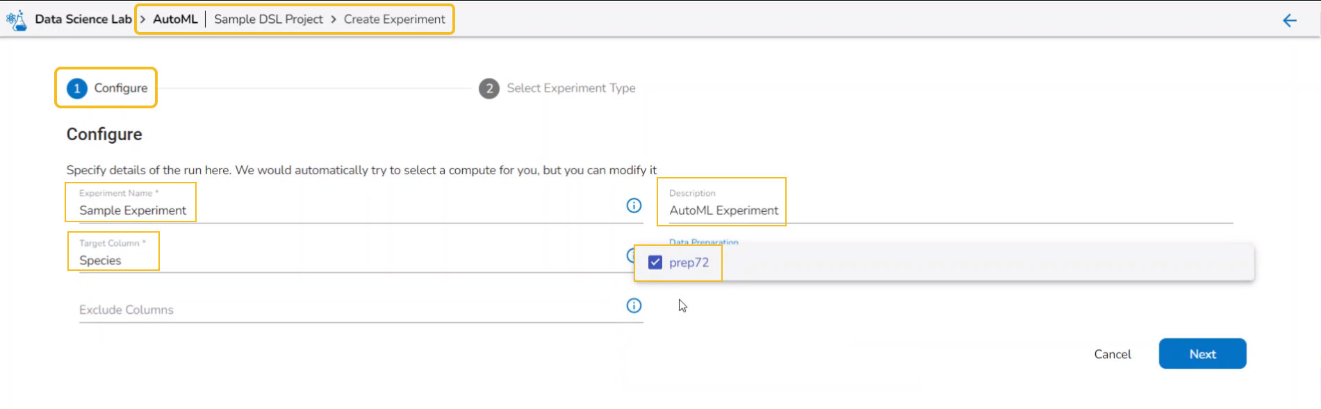
The Configure tab opens (by default) while selecting the Create Experiment option.
Provide the following information:
Provide a name for the experiment.
The user gets redirected to the Select Experiment Type tab.
Select a prediction model using the checkbox.
Based on the selected experiment type a validation notification message appears.
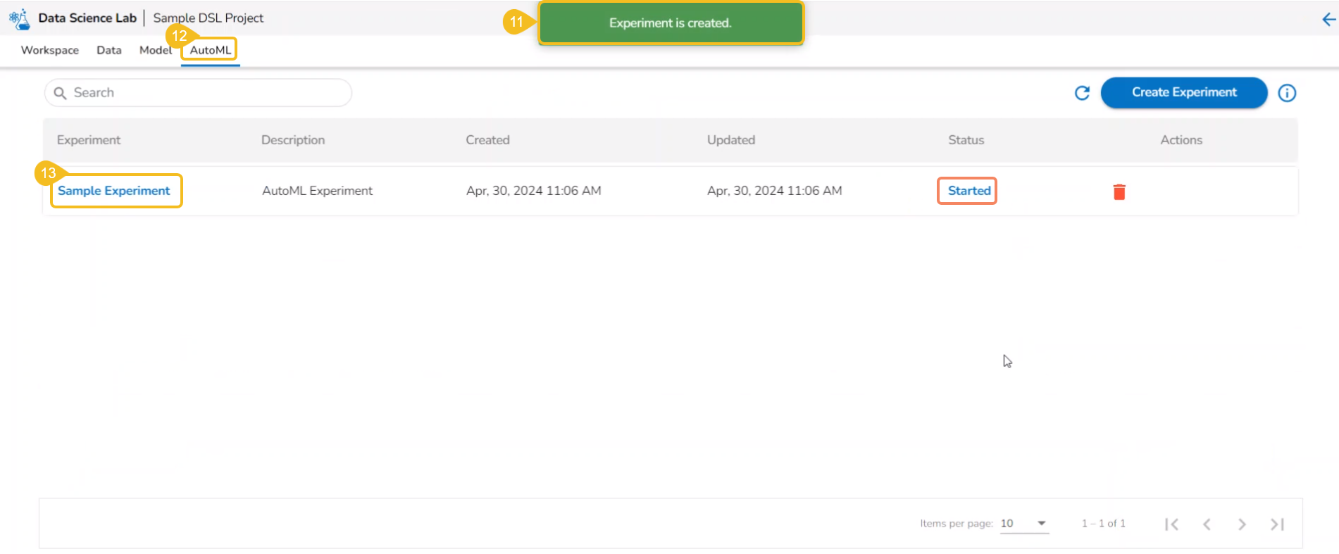
A notification message appears.
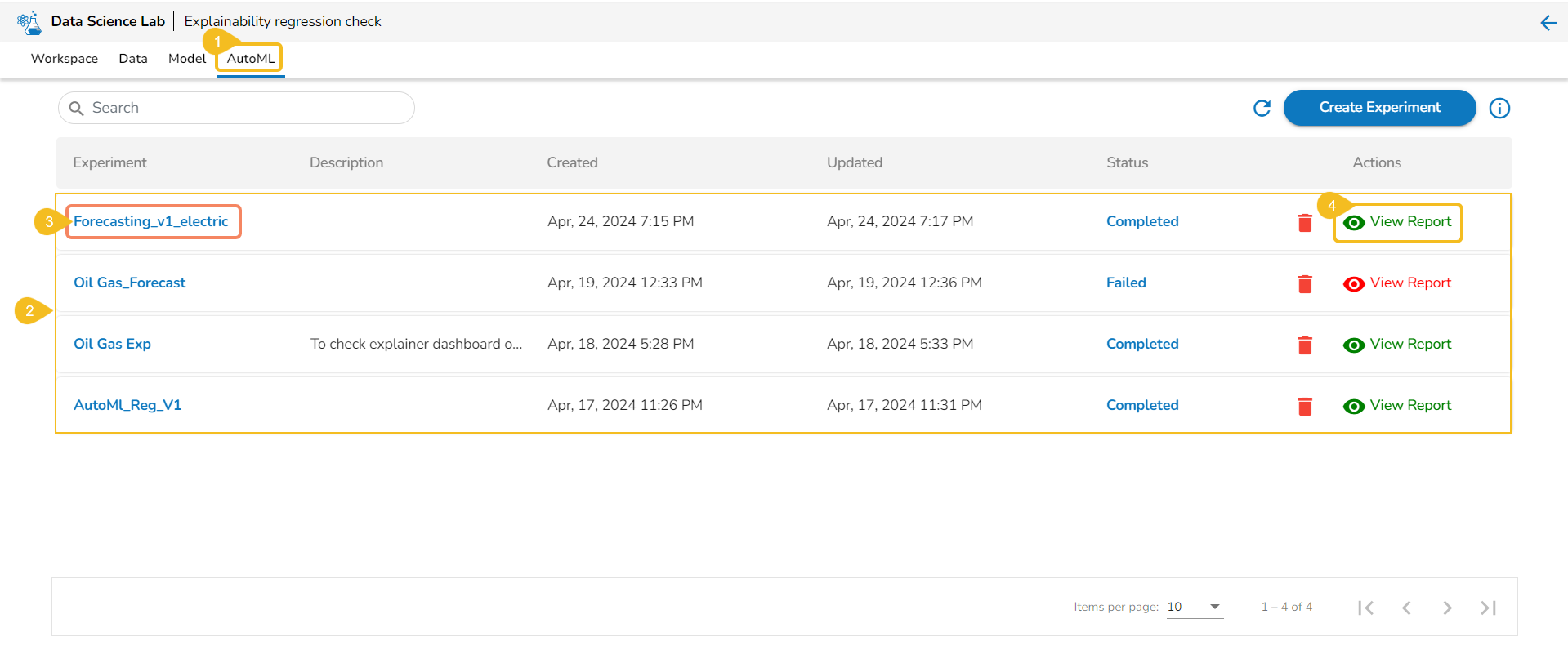
The user is redirected to the AutoML list page.
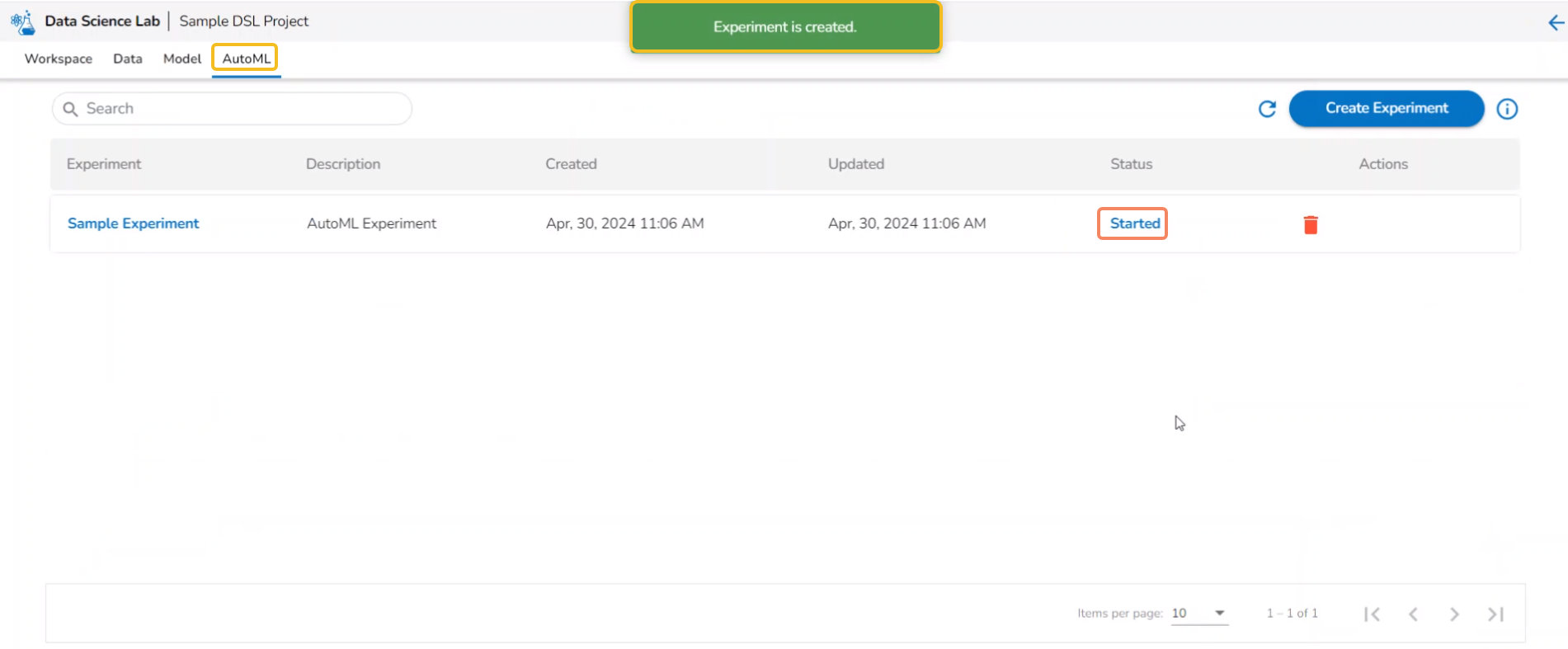
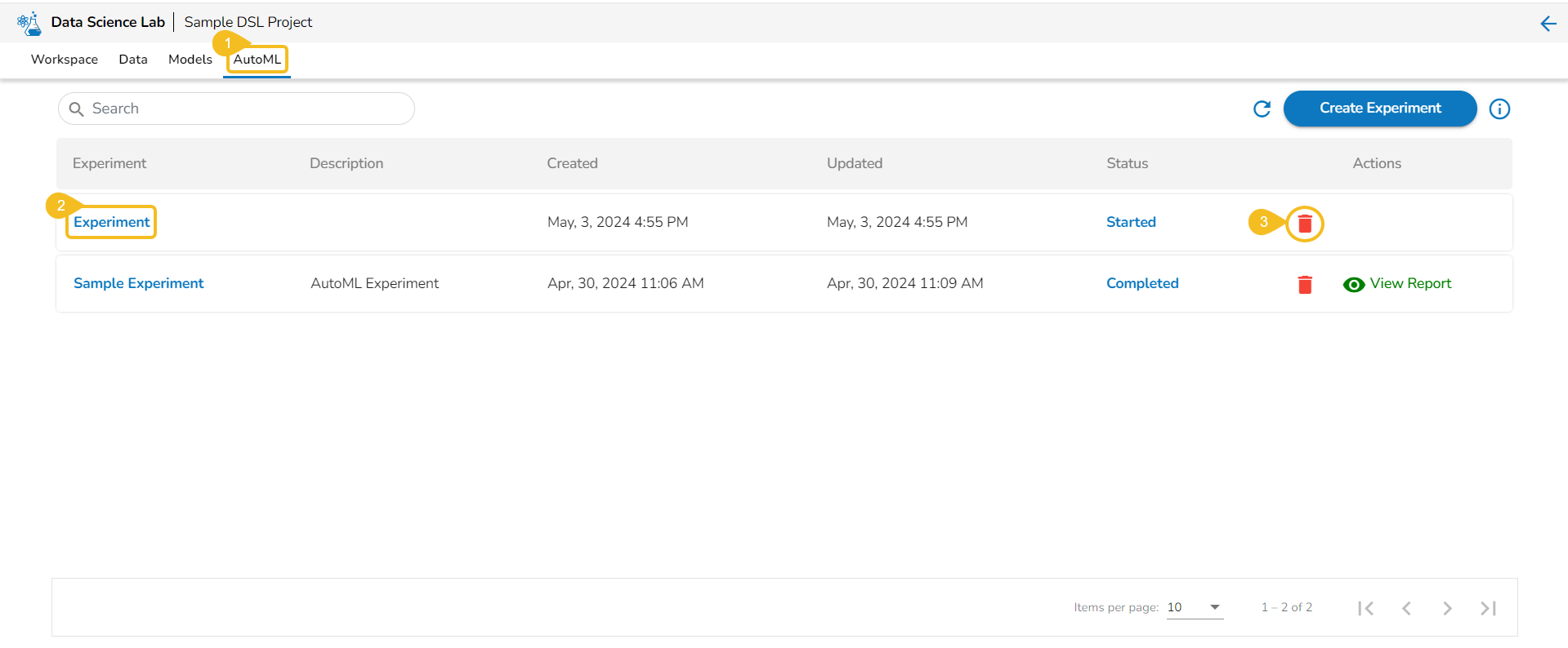
The newly created experiment gets added to the list with Status mentioned as Started.
Various Status of a Created Experiment
The Status tab indicates various phases of the experiments/model training. The different phases for an experiment are as given below:
The newly created experiment gets Started status. It is the first status when a new experiment is created.
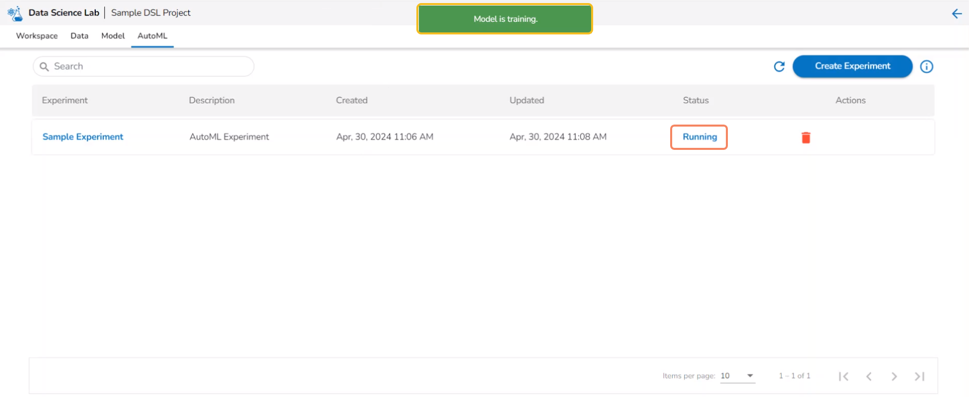
Another notification message appears to inform the user that the model training has started. The same is indicated through the Status column of the model. The Status for such models will be Running.
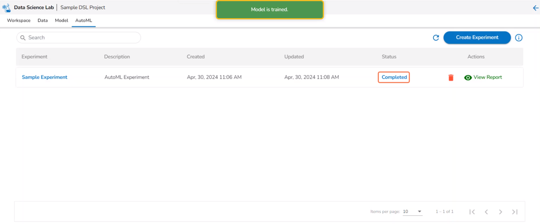
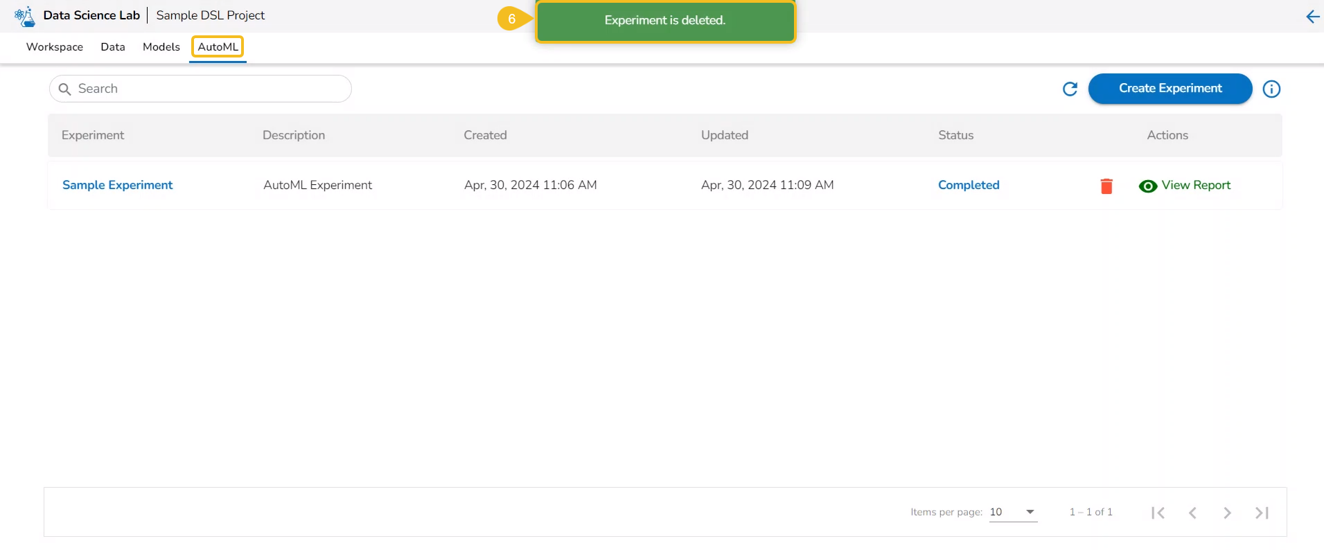
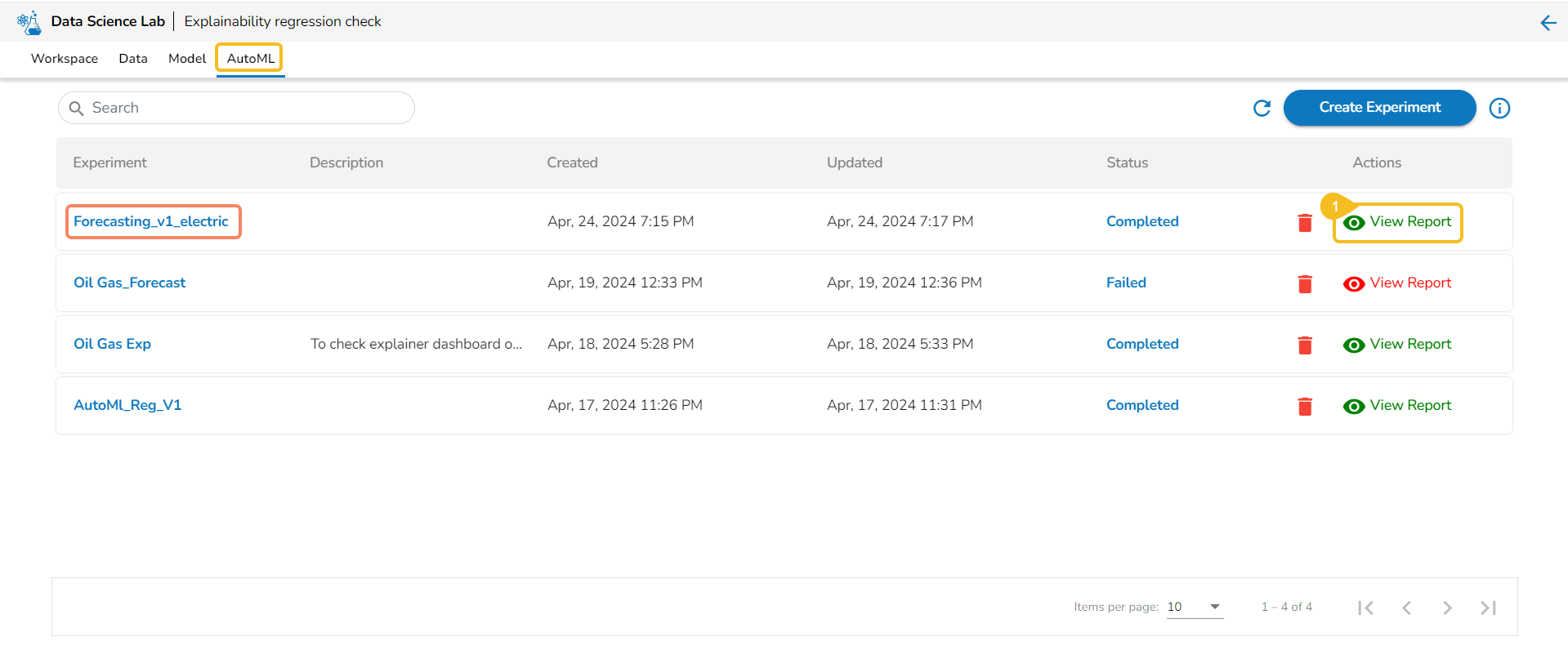
After the experiment is completed, a notification message appears stating that the model trained. The Status for a trained model will be indicated as Completed.
Please Note: The unsuccessful experiments are indicated as Failed under the status. The View Report is mentioned in red color for the Failed experiments.
Using a Markdown Cell
This page describes steps to use the text cells of the Data Science Notebook.
The Markdown cells are used to enter a description, links, images, headings, and text with Bold or Italics effect to a Data Science Notebook. They are formatted using a simple markup language called Markdown. The Markdown cell contains a toolbar to assist with editing.
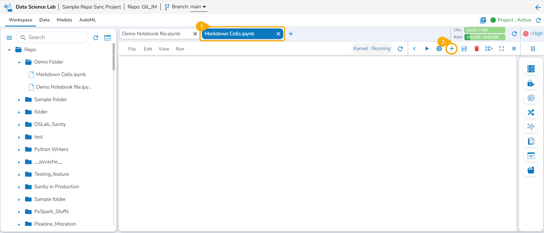
Inserting a Markdown Cell
Navigate to a .ipynb file.
Use the Add pre-cell icon to insert a new code cell to the file.
OR
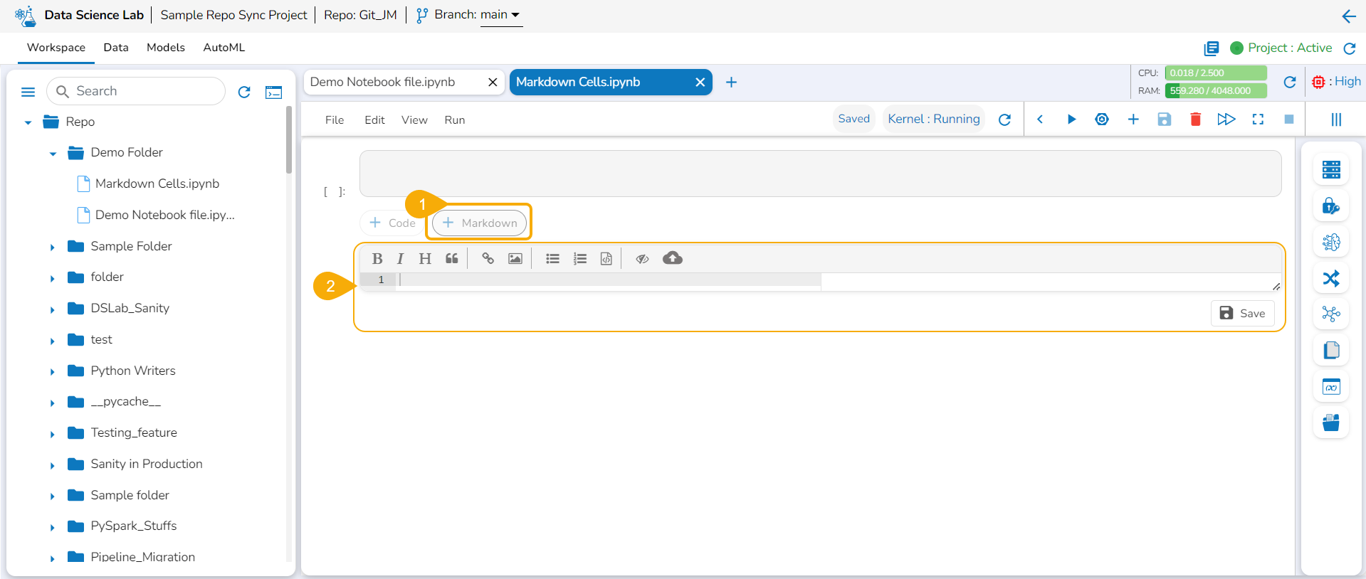
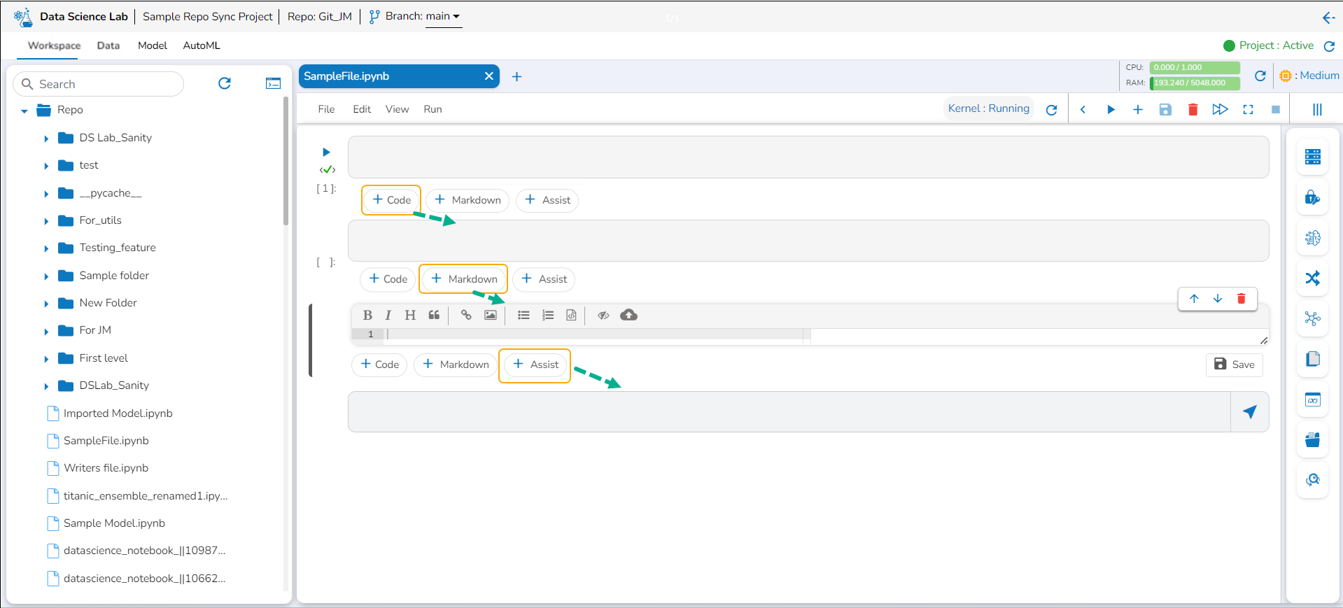
Click the +Markdown option that appears below the code cell.
The Markdown cell appears below to insert Markdown into the Notebook.
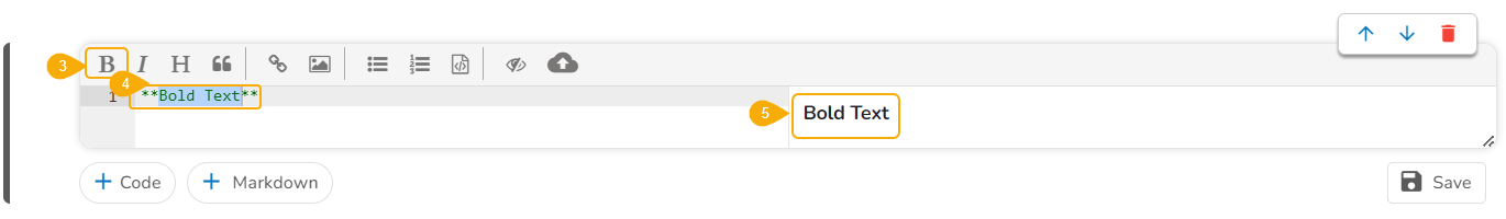
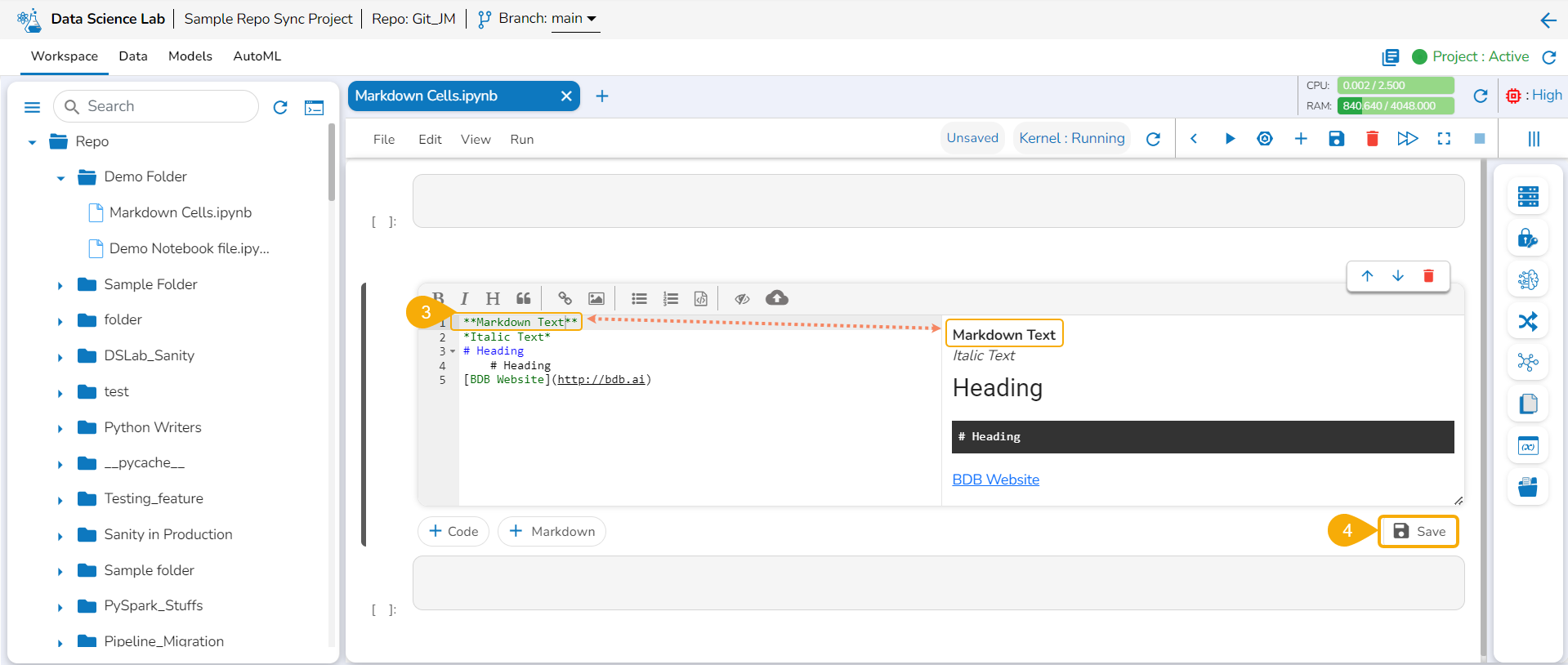
Choose an action from the toolbar.
It gets added to the left side of the Markdown cell.
The right-side Markdown space displays the text with the applied effect.
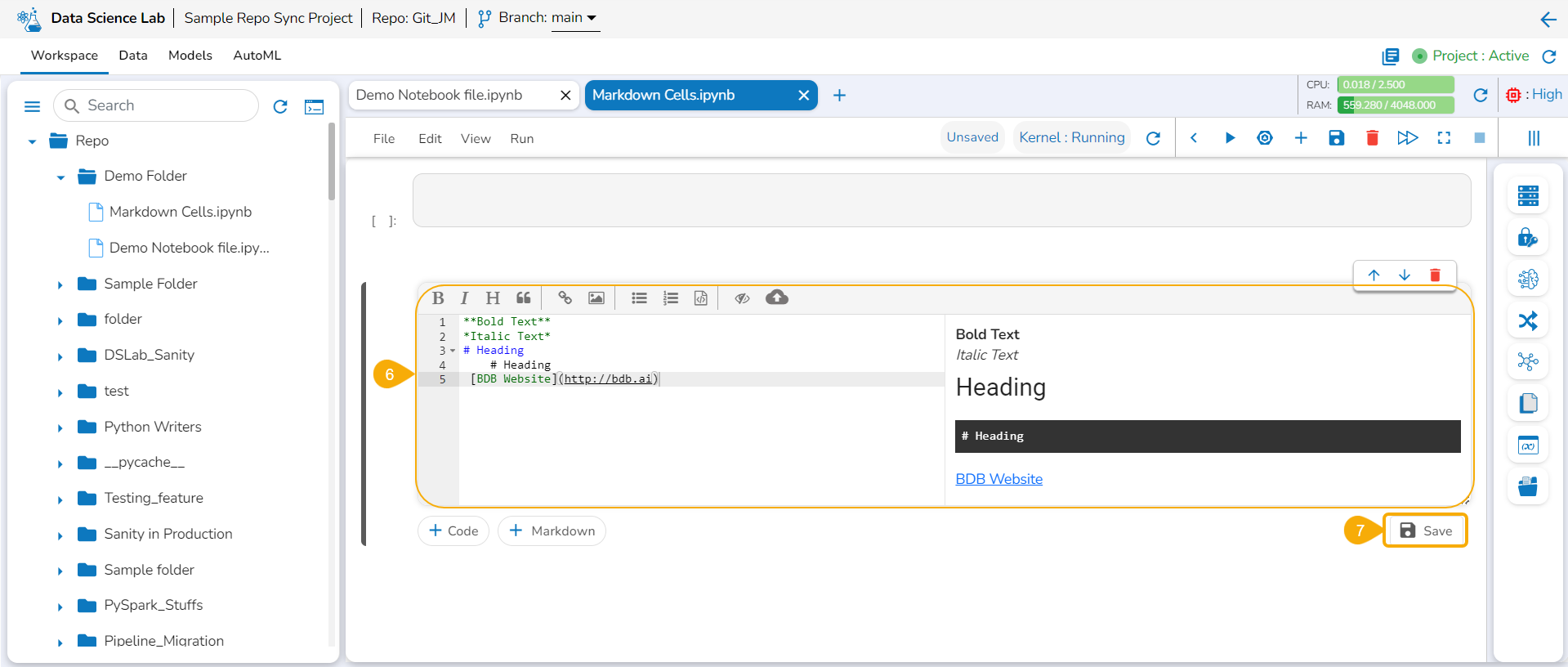
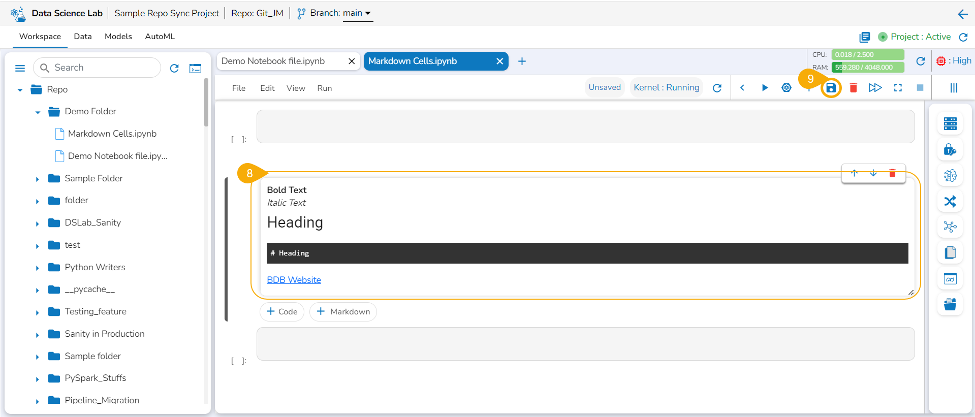
The image displays a few actions from the toolbar (such as Bold, Italic, Heading, and link) applied to the Markdown text.
Click the Save option.
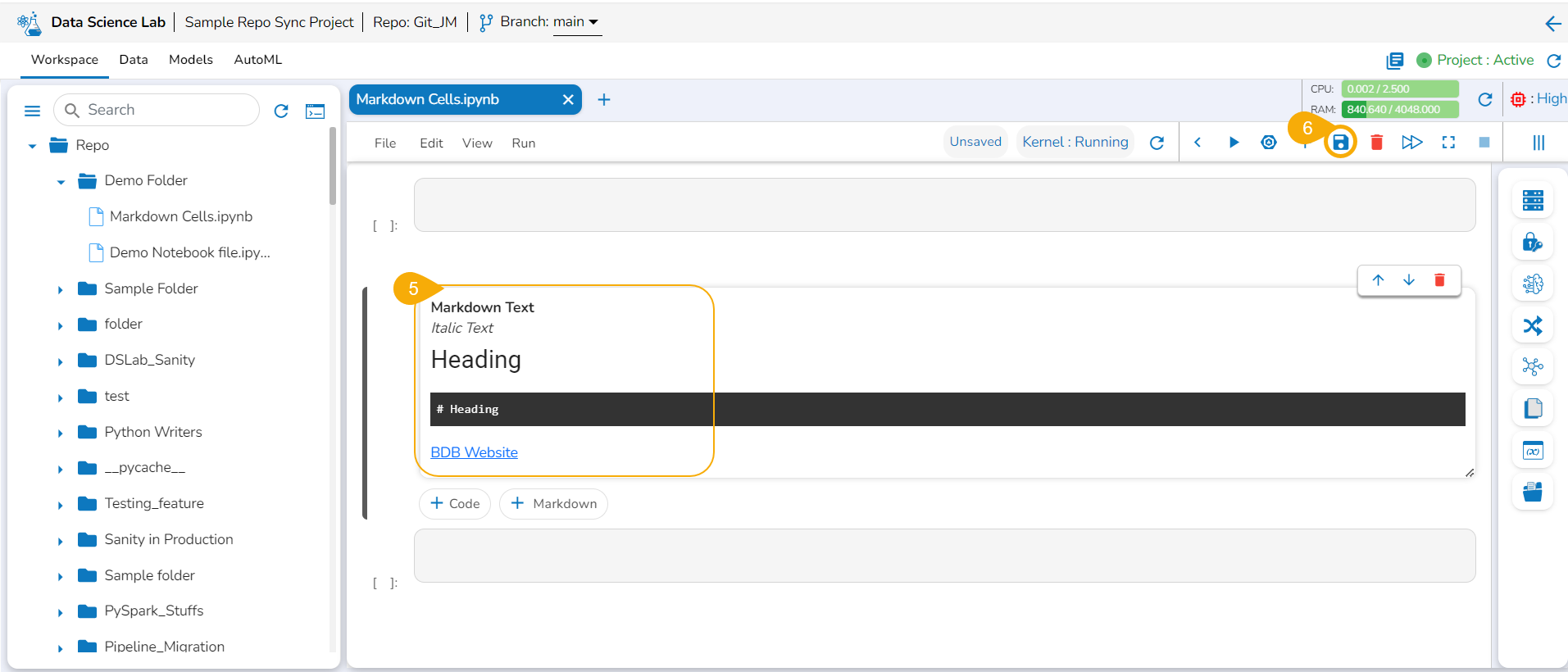
The Markdown cell with inserted effect gets saved and the Markdown display gets changed displaying the text with saved effects on the left side (as shown in the given image).
Please Note: A Code cell gets added below the saved Markdown cell.
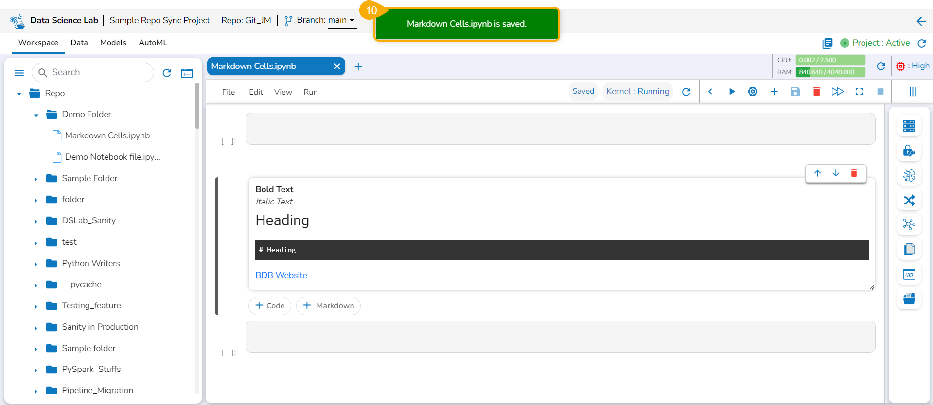
The user can click the Save option provided for the Notebook to save the update in the Notebook (after the Markdown cell has been added to it).
The Notebook gets updated and the same gets communicated through a notification message.
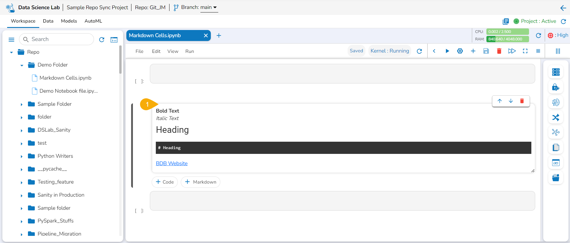
Editing a Markdown Cell
Use the double clicks on a saved Markdown cell.
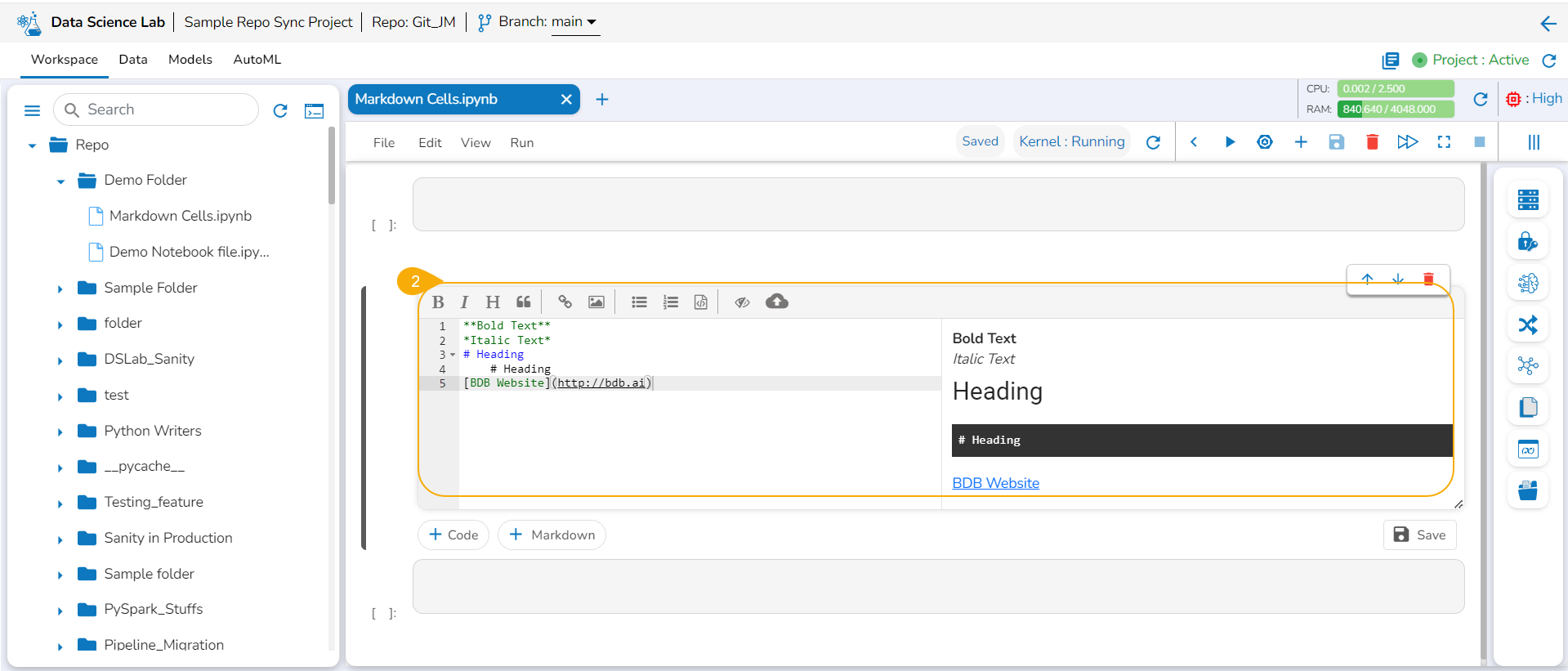
The Markdown cell opens in the editable format to edit it.
Modify the text inside the Markdown cell.
Click the Save option to update the edited Markdown in the Notebook.
Click the Save option for the file.
A notification message appears.
The file gets saved with the Markdown cell.
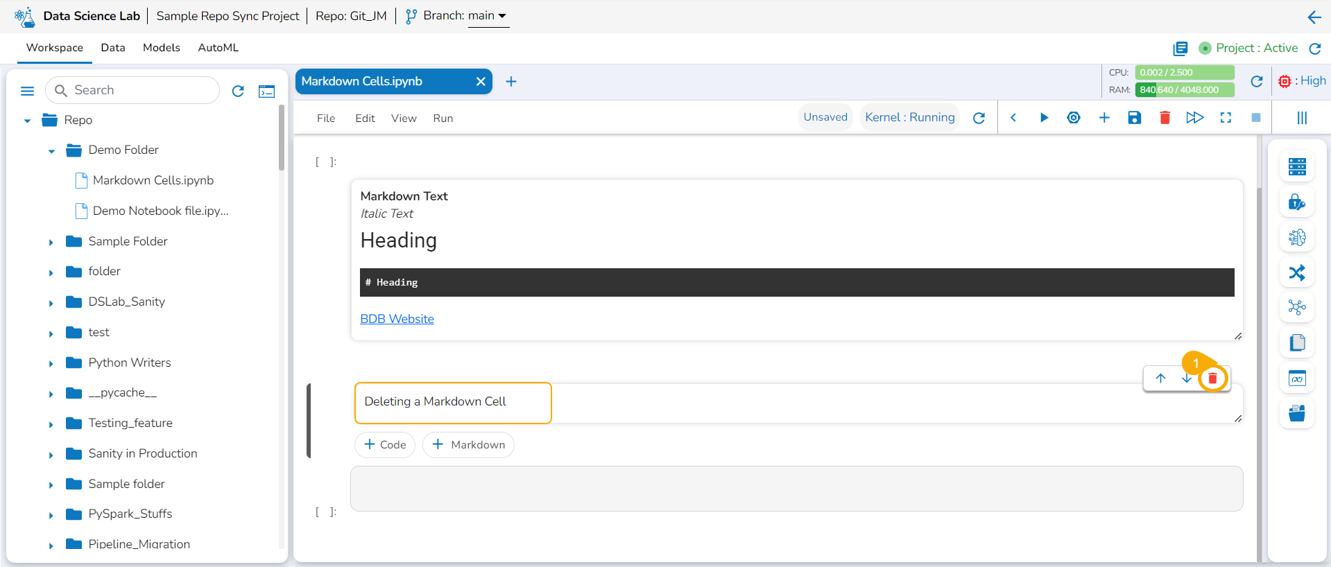
Deleting a Markdown Cell
Click the Delete markdown icon for a saved Markdown cell.
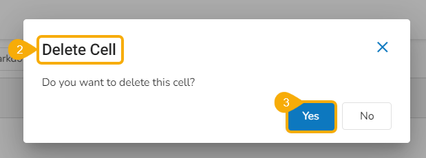
The Delete Cell dialog box opens.
Click the Yes option.
The selected Markdown gets removed and the same gets communicated by a notification message.
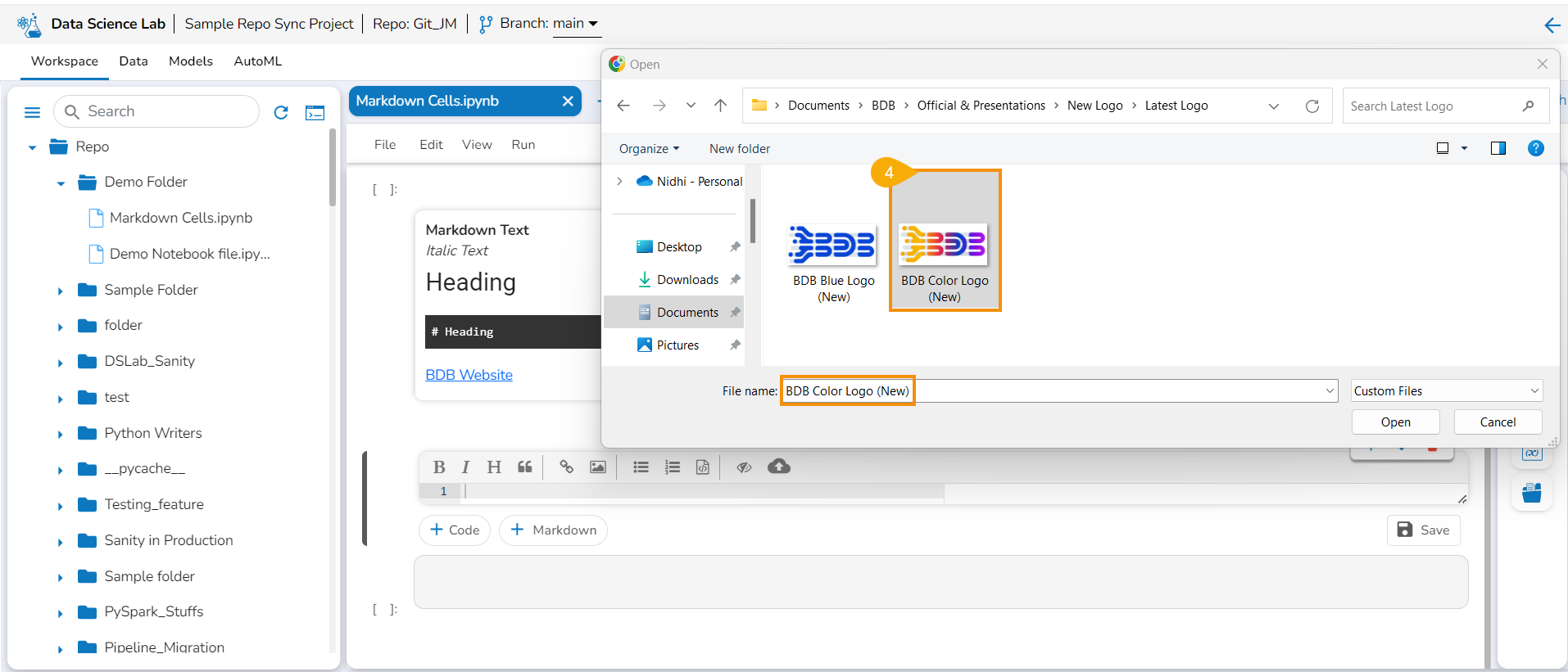
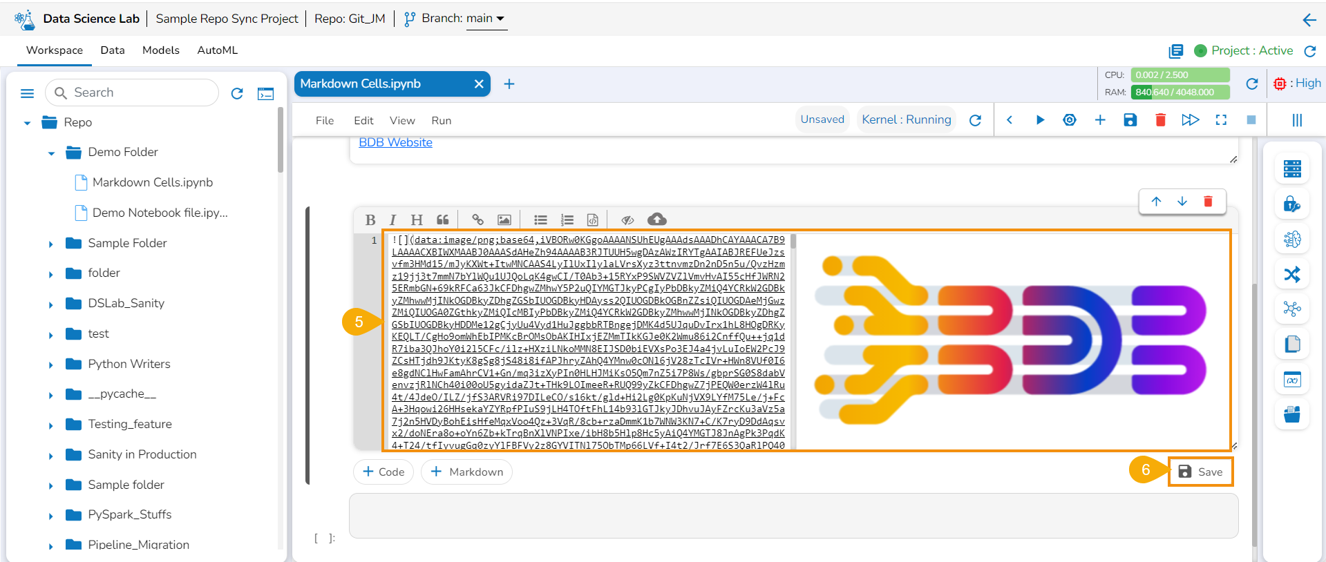
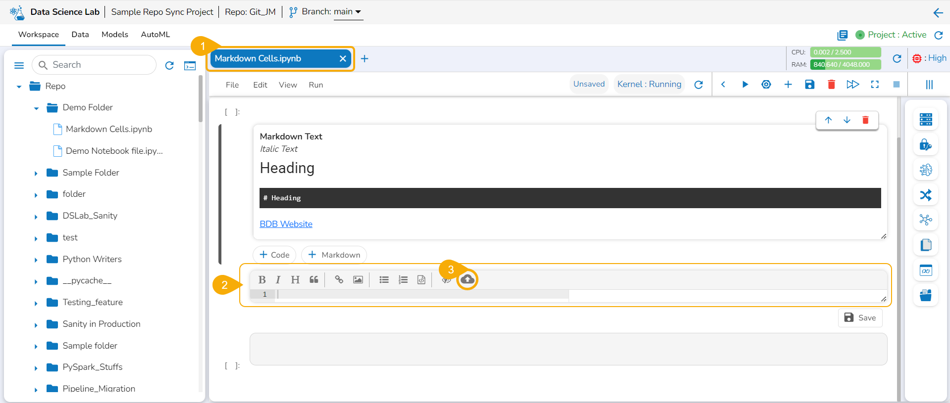
Uploading an Image in the Markdown
Navigate to a .ipynb file inside an activated Project.
Access a Markdown cell.
Click the Upload icon.
Upload an image.
The image gets uploaded to the markdown cell.
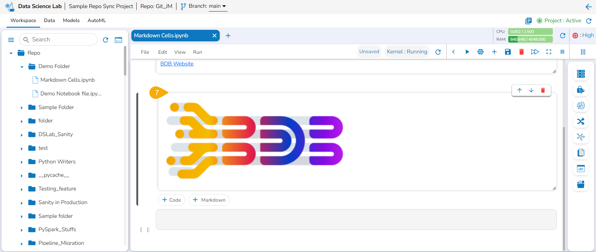
Click the Save icon.
The markdown cell gets saved the uploaded image appears in the View mode of the markdown.
Please Note: Do not forget to click the Save icon for the Data Science Notebook to save the markdown updates in the .ipynb file.
Create
The Create option redirects the user to create a new Notebook under the selected Project.
Check out the illustration on creating a new Notebook inside a DSL Project.
Please Note: The Create option appears for the Repo folder that opens by default under the Workspace tab.
Creating a New Notebook
Navigate to the Workspace tab for a Data Science Lab project.
Click the Create option from the Notebook tab.
Please Note: The Create option gets enabled only if the Project status is Active as mentioned in the above-given image.
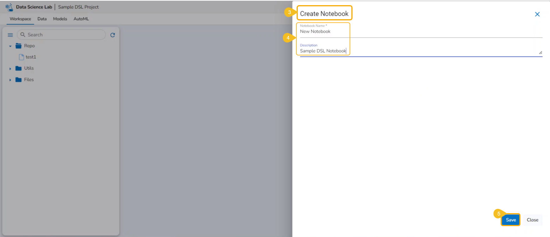
The Create Notebook page opens.
Provide the following information to create a new Notebook:
Notebook Name
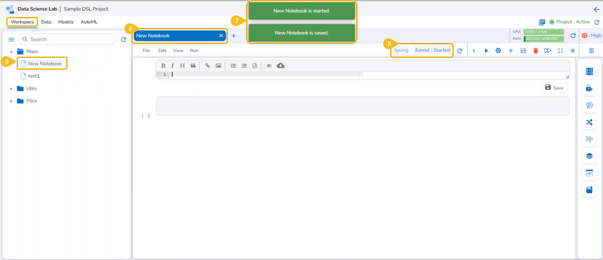
The Notebook gets created with the given name and the Notebook page opens. The Notebook may take a few seconds to save and start the Kernel.
The user will get notifications to ensure the new Notebook has been saved and started.
The same gets notified on the Notebook header (as highlighted in the image).
Adding a New Notebook
Check out the illustration on adding a new Notebook.
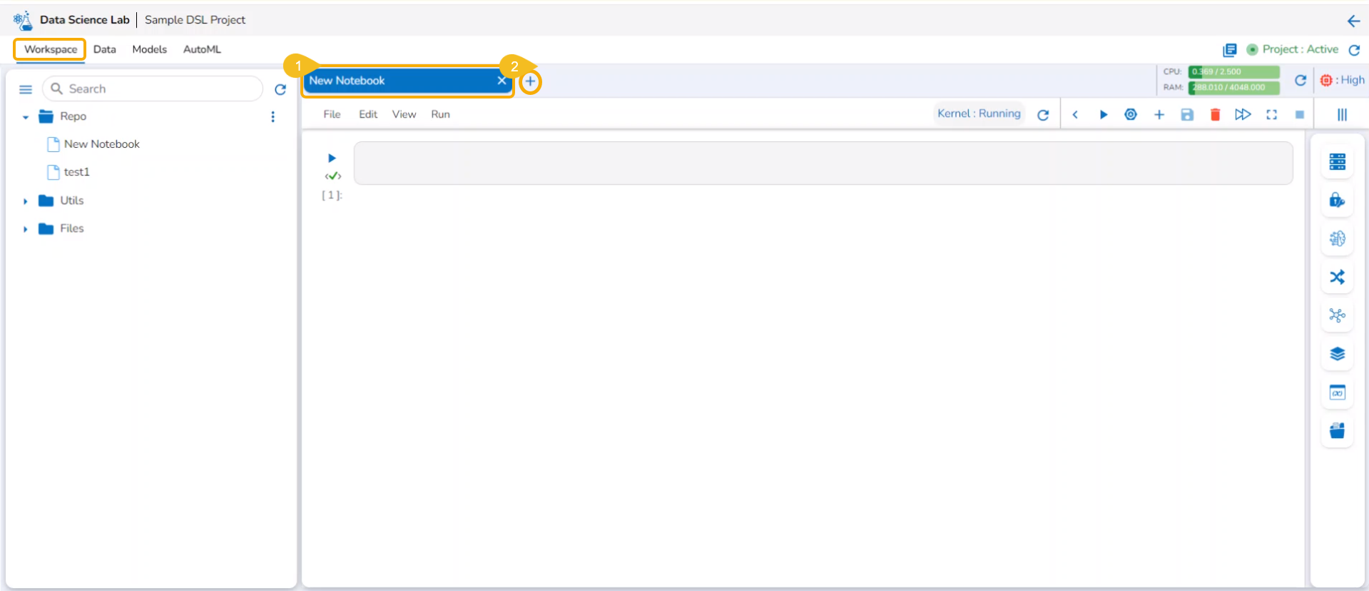
The users also get an Add option to create a new Notebook. This option becomes available to the users only after at least one Notebook is created using the Create option and open it.
Open an existing Notebook from a Project.
The Add icon appears on the header next to the opened Notebook name. Click the Add icon.
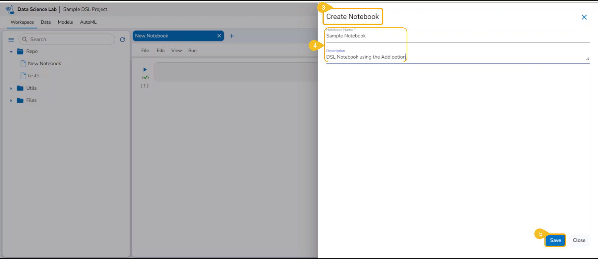
The Create Notebook window opens.
Provide the Notebook Name and Description.
Click the Save option.
A new Notebook gets created and the user will be redirected to the interphase of the newly created Notebook.
Soon the notification messages assuring the user that the newly created Notebook has been saved and started appear on the screen.
The Notebook gets listed under the Notebook list provided on the left side of the screen.
A code cell gets added by default to the newly created Notebook for the user to begin the data science experiment.
Please Note:
The user can edit the Notebook name by using the Edit Notebook Name icon.
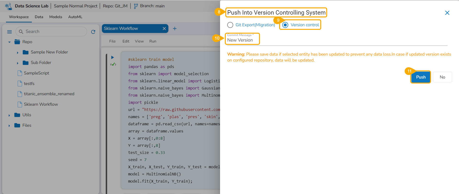
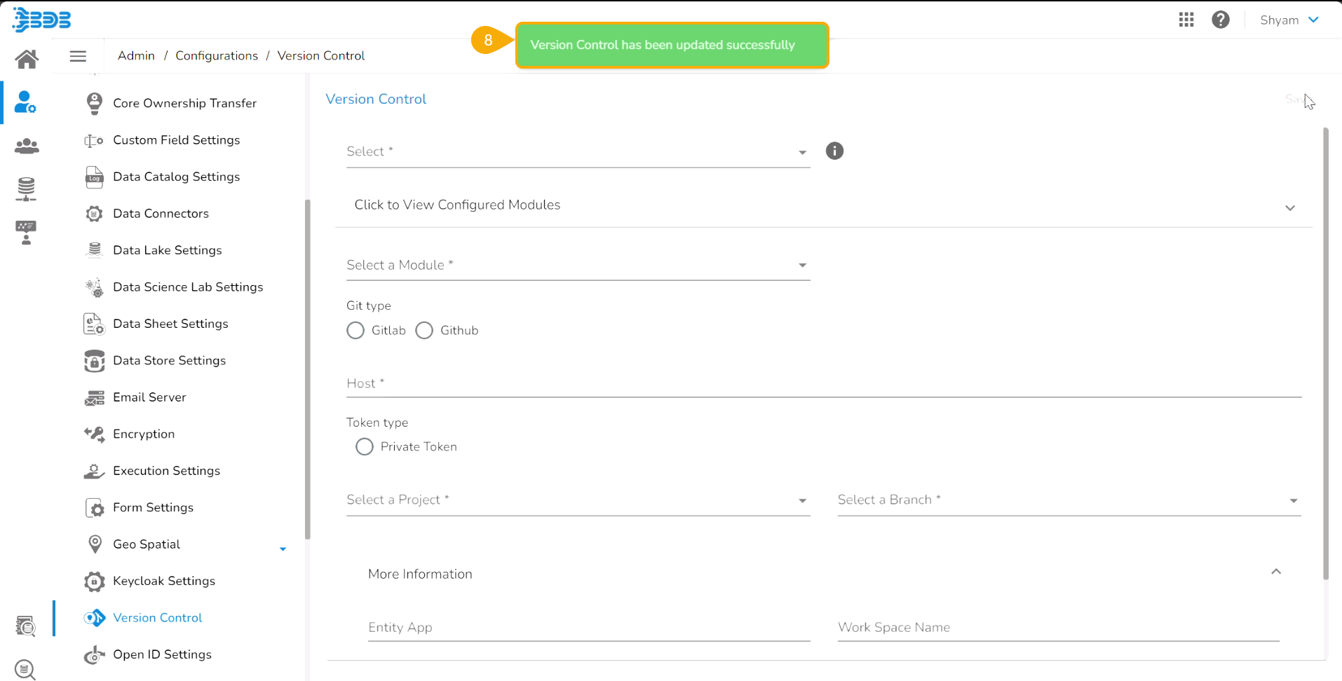
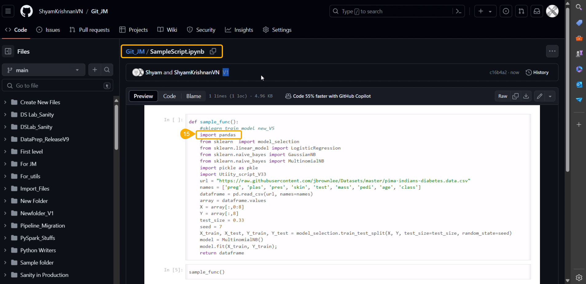
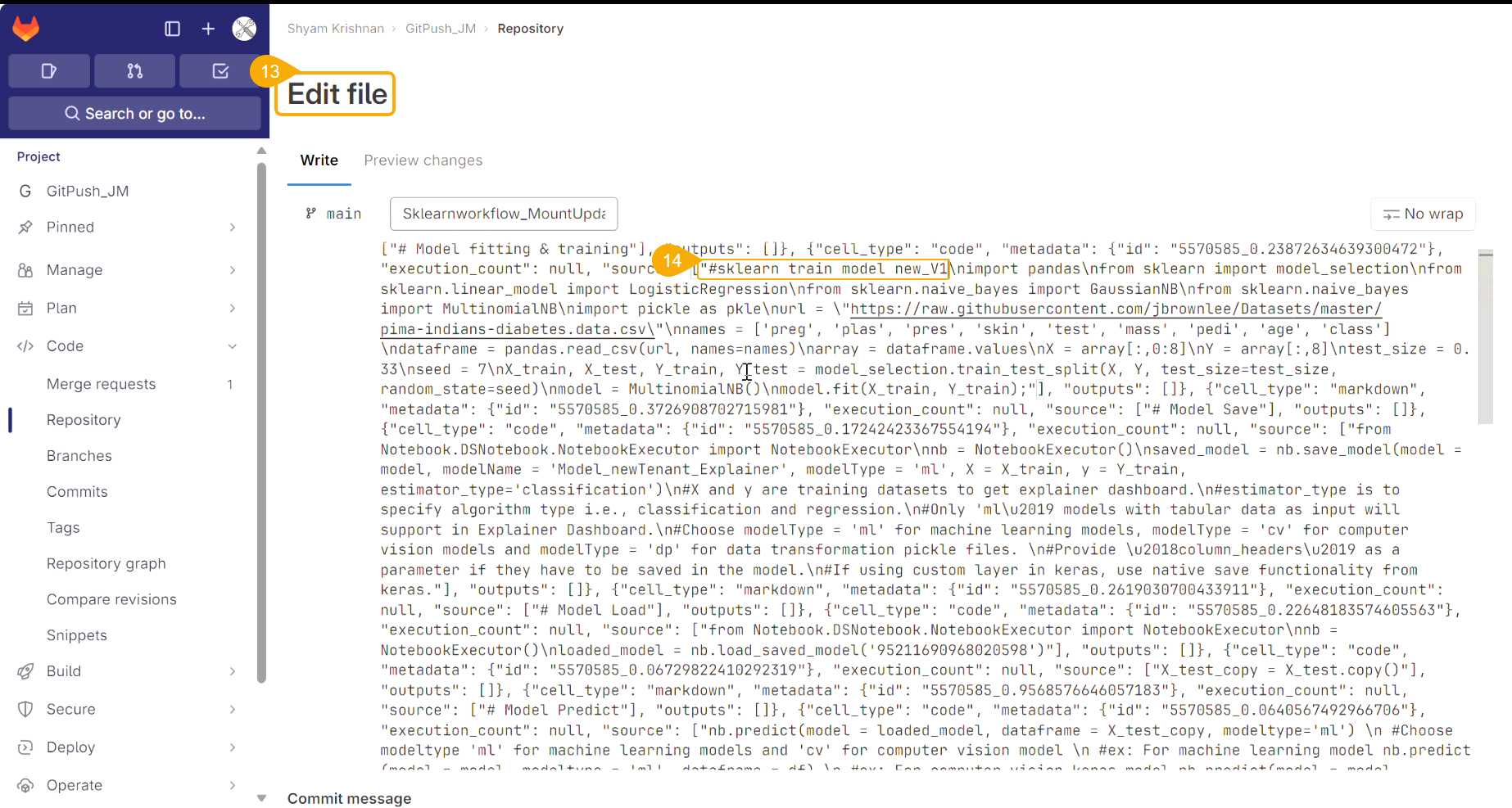
Export to GIT/ Model Migration
This page explains Model migration functionality. You can find steps to Export and Import a model to and from Git repository explained on this page.
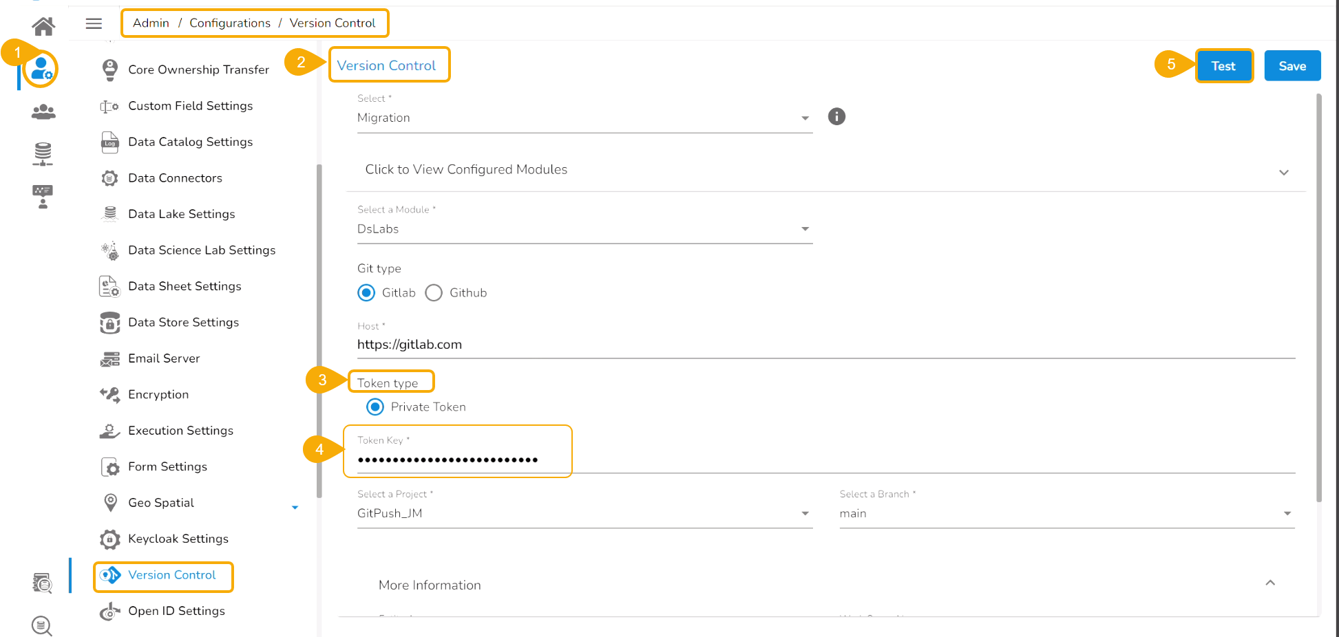
Prerequisite: The user must do the required configuration for the DS Lab Migration using the Admin module before migrating a DS Lab script or model.
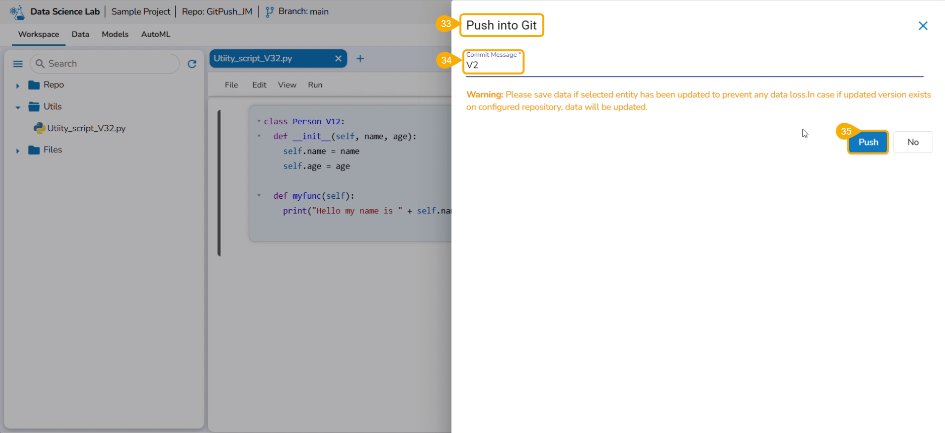
Export a DSL Model to GIT
The user can use the Migrate Model icon to export the selected model to the GIT repository.
Check out the illustration on Export to Git functionality.
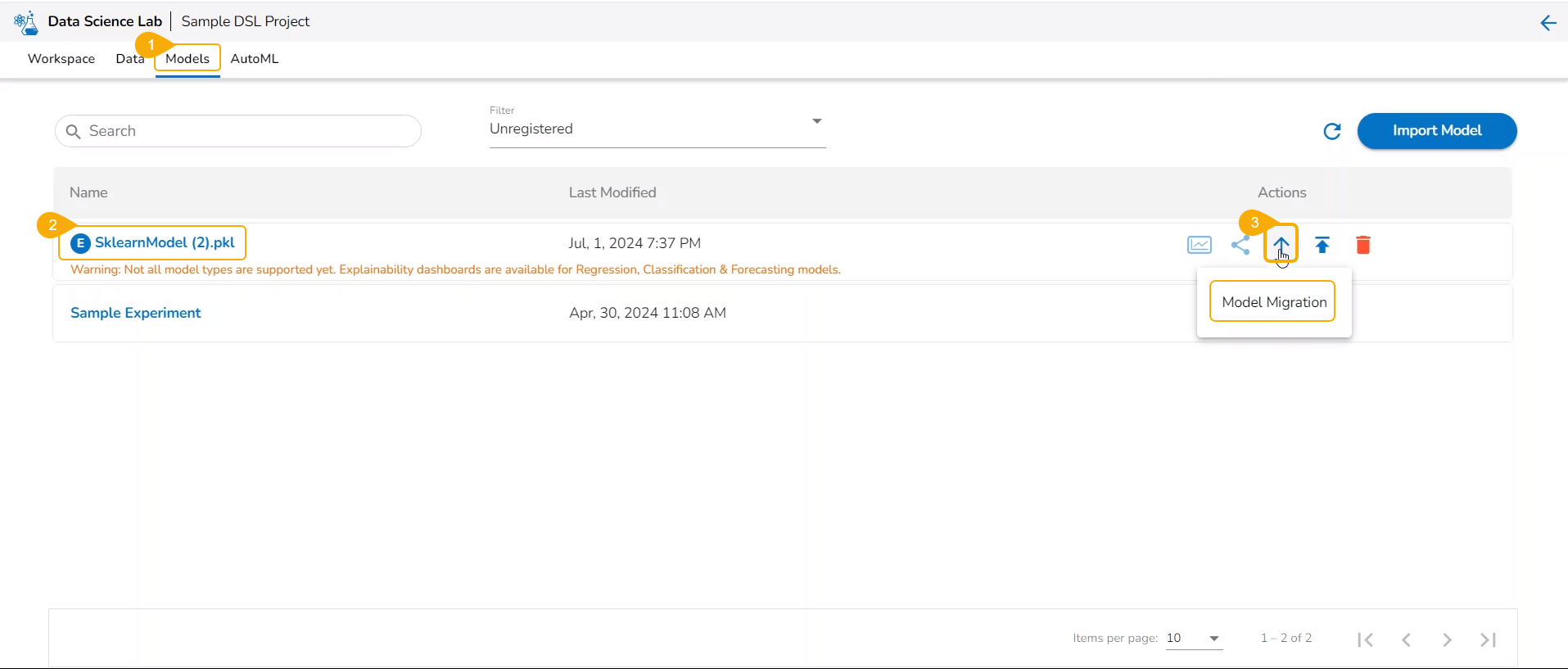
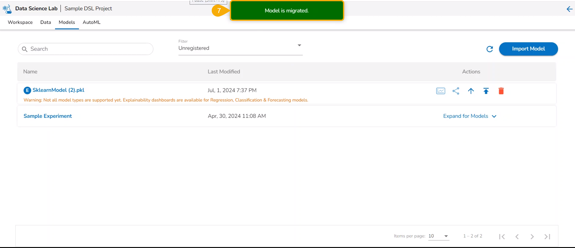
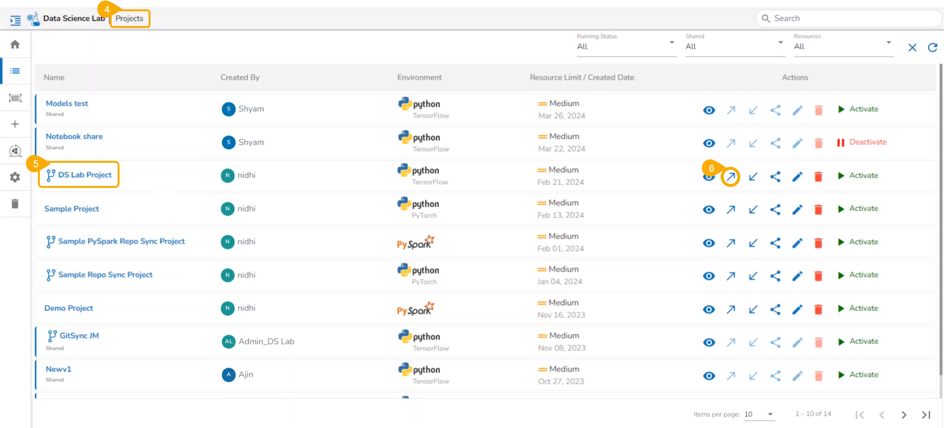
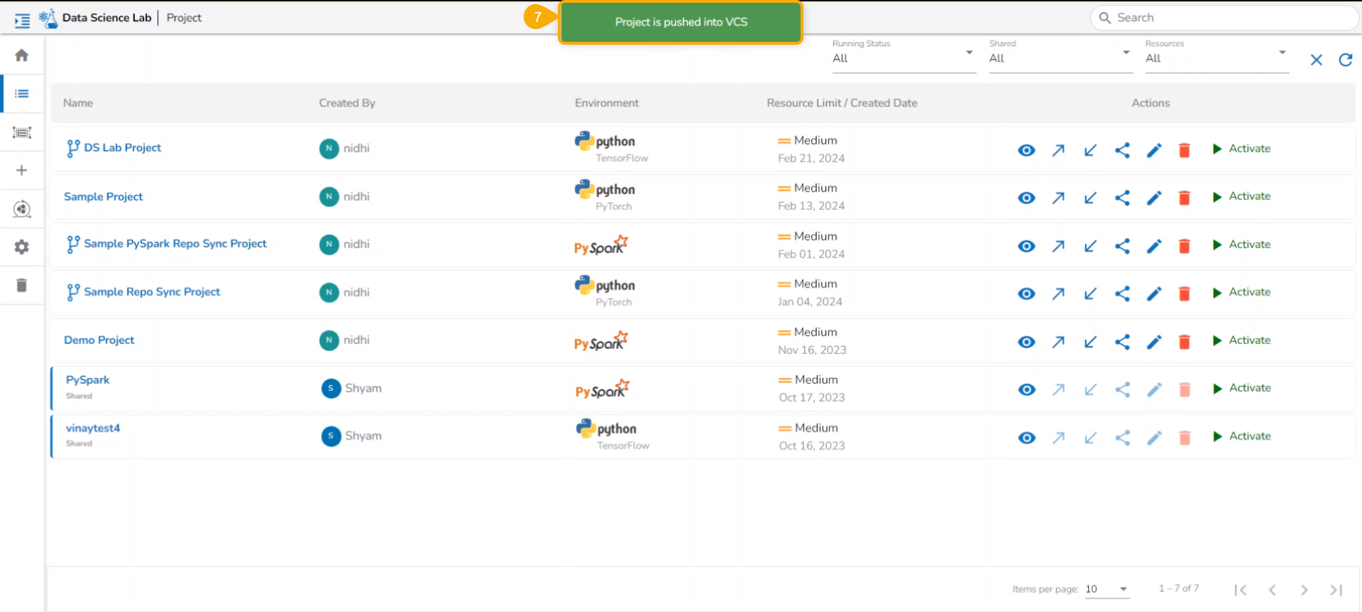
Navigate to the Models tab.
Select a model from the displayed list
Click the Model Migration icon for a Model.
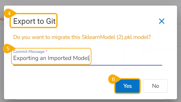
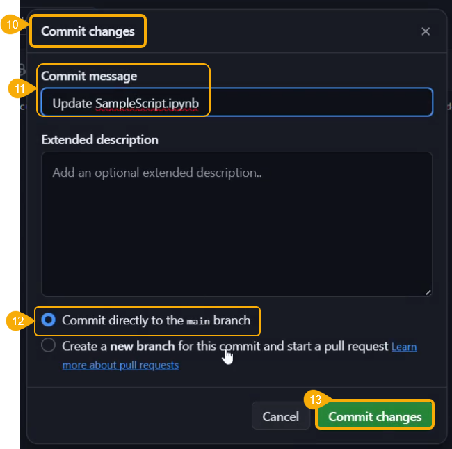
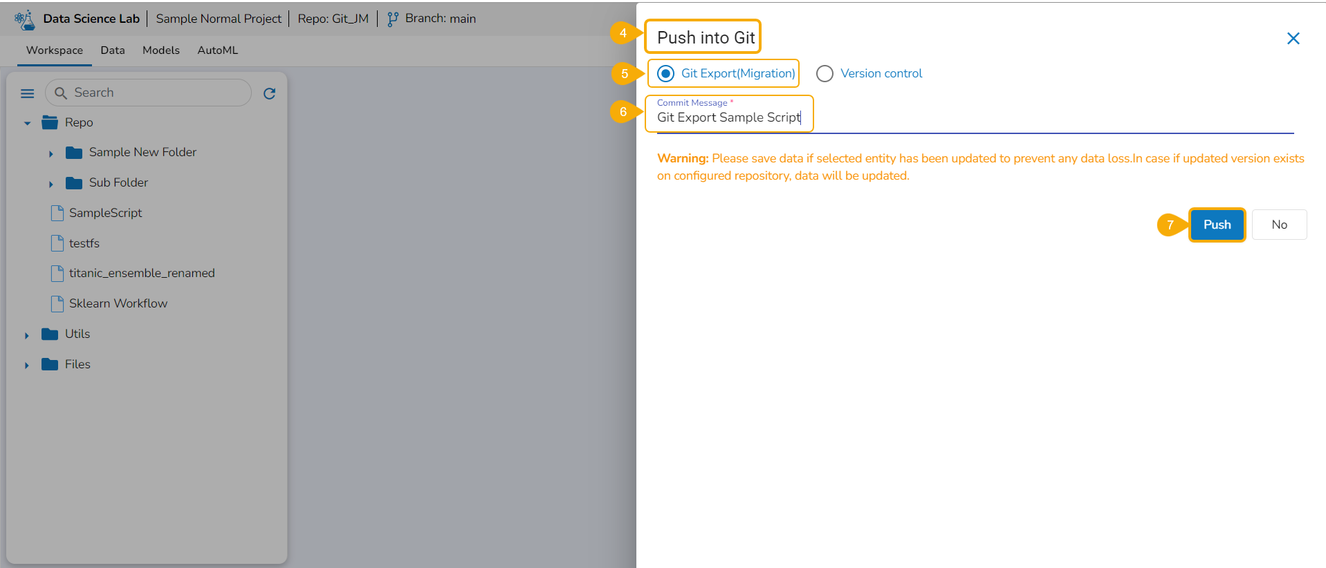
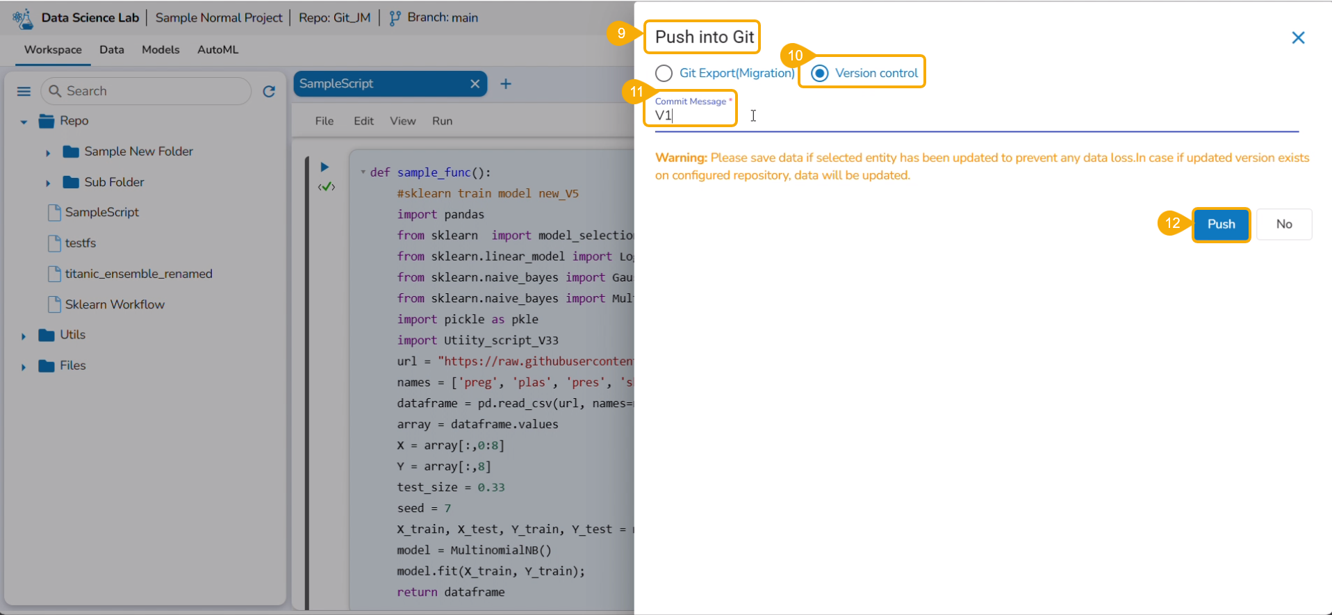
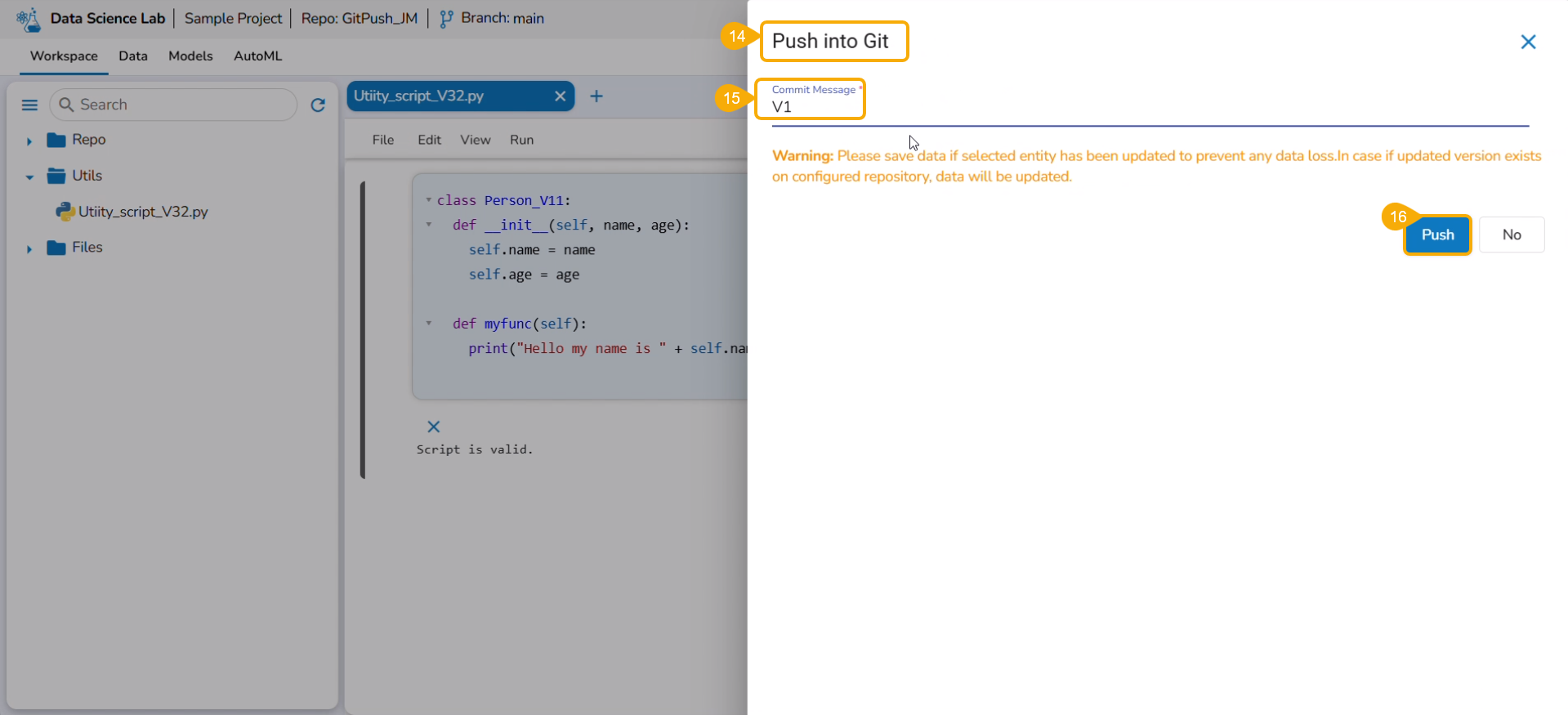
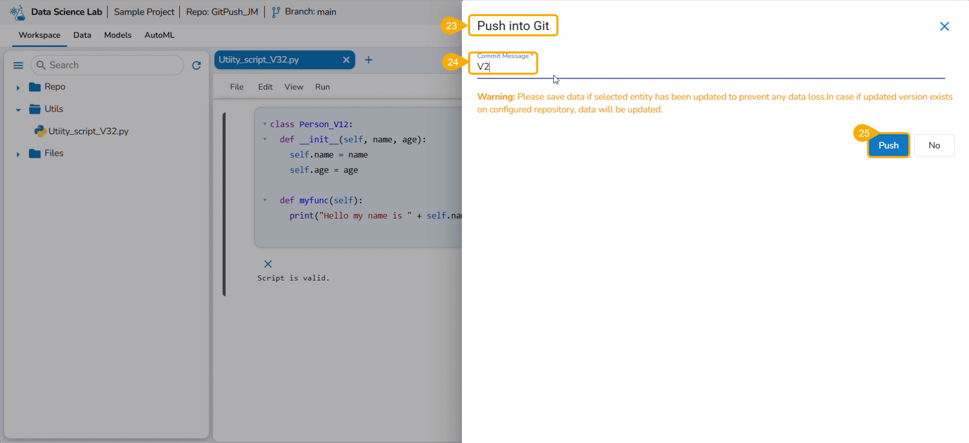
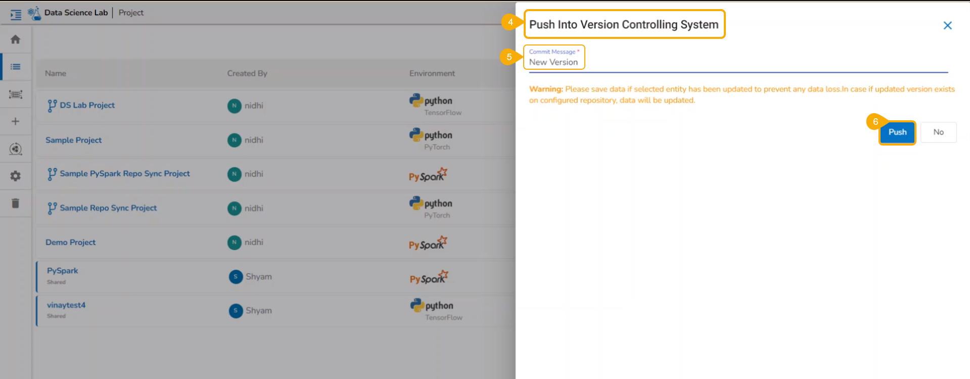
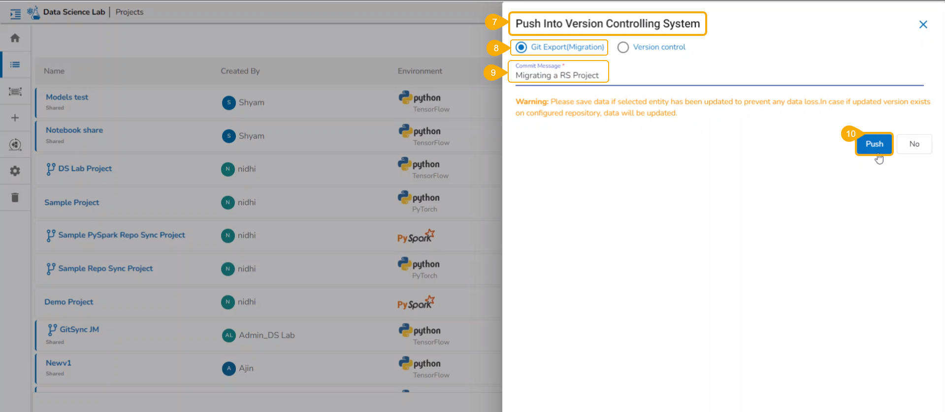
The Export to GIT dialog box opens.
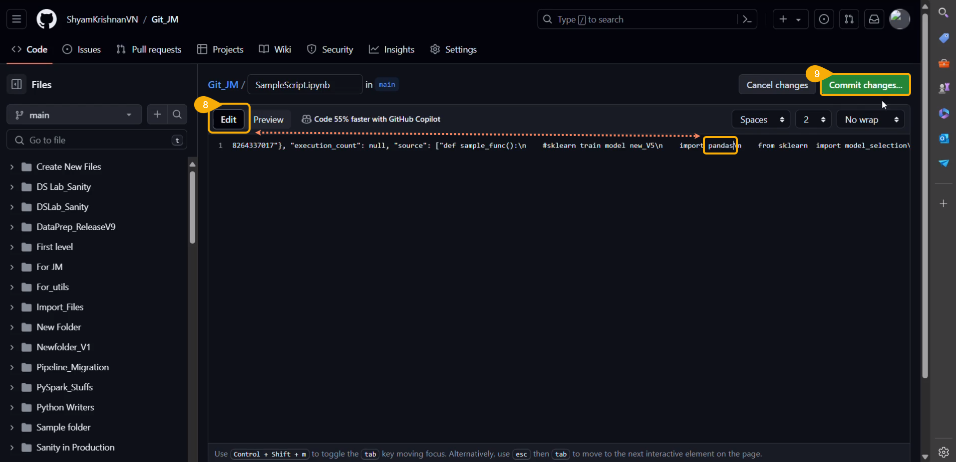
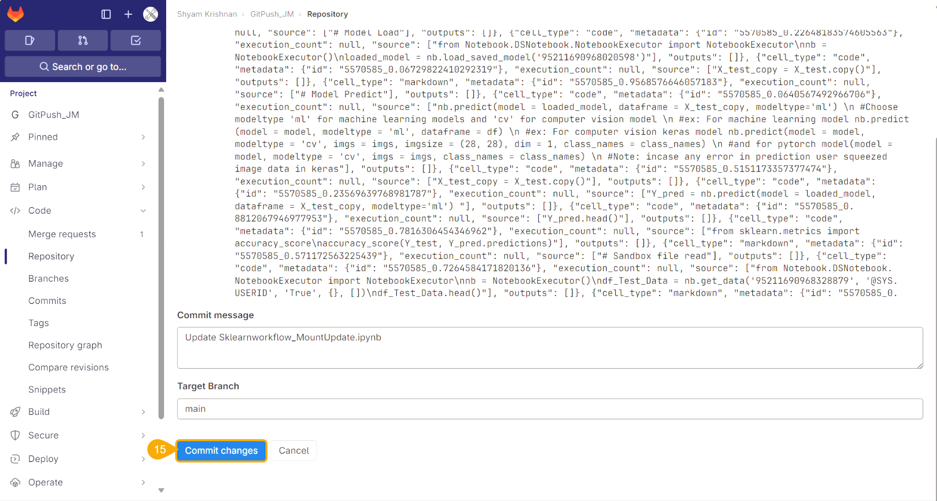
Provide a Commit Message in the given space.
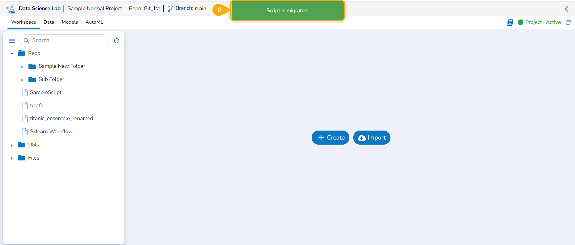
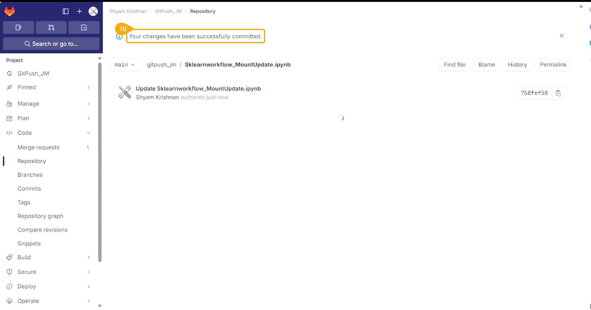
Click the Yes option.
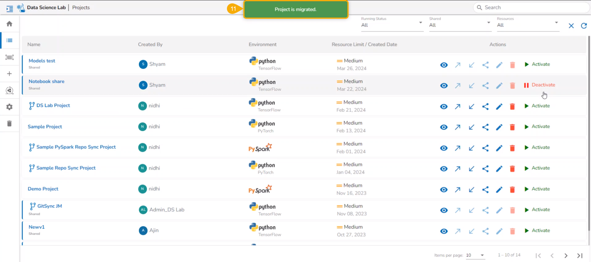
A notification message appears informing that the model is migrated.
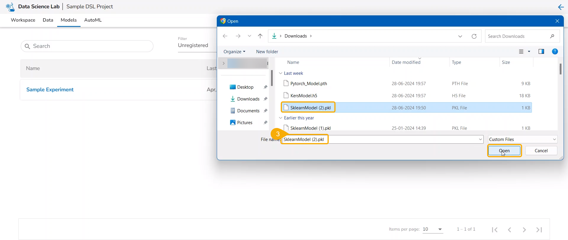
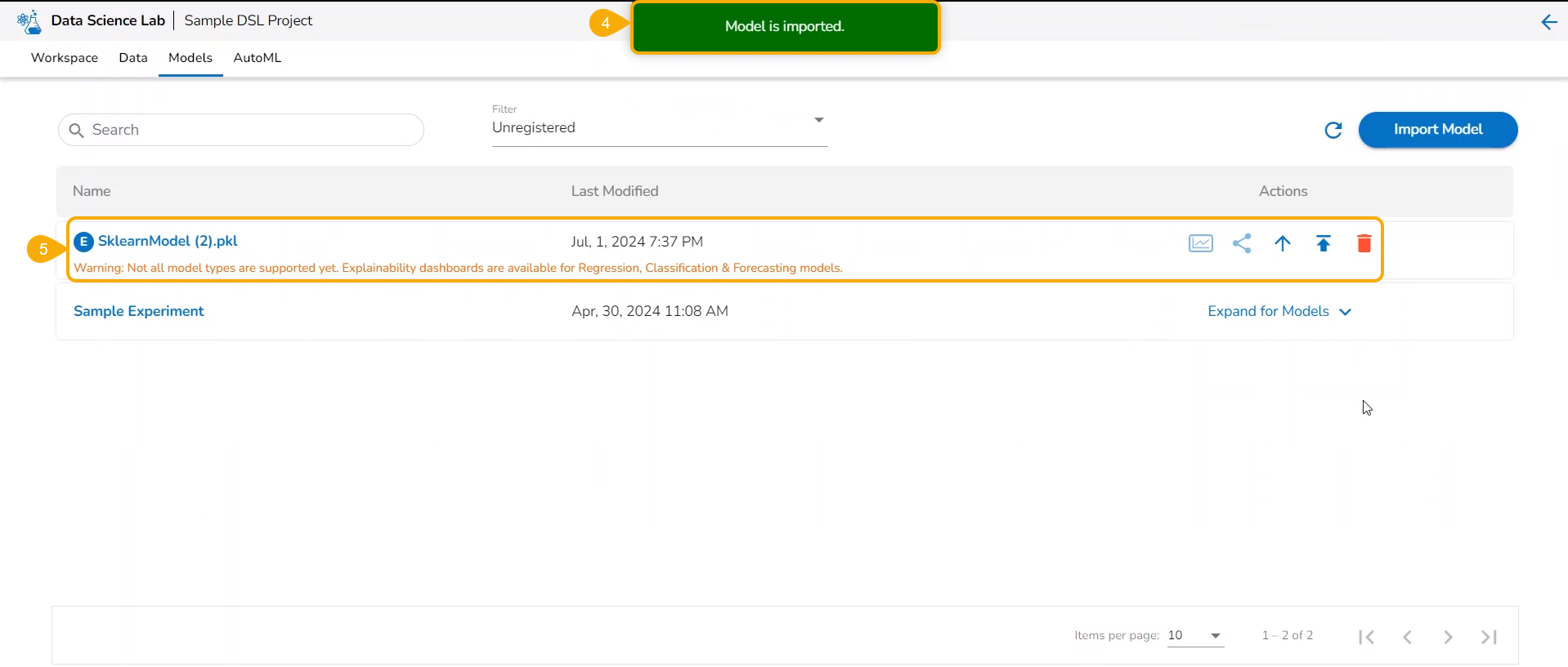
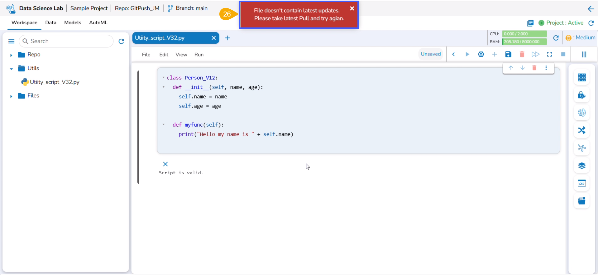
Import a DSL Model from GIT
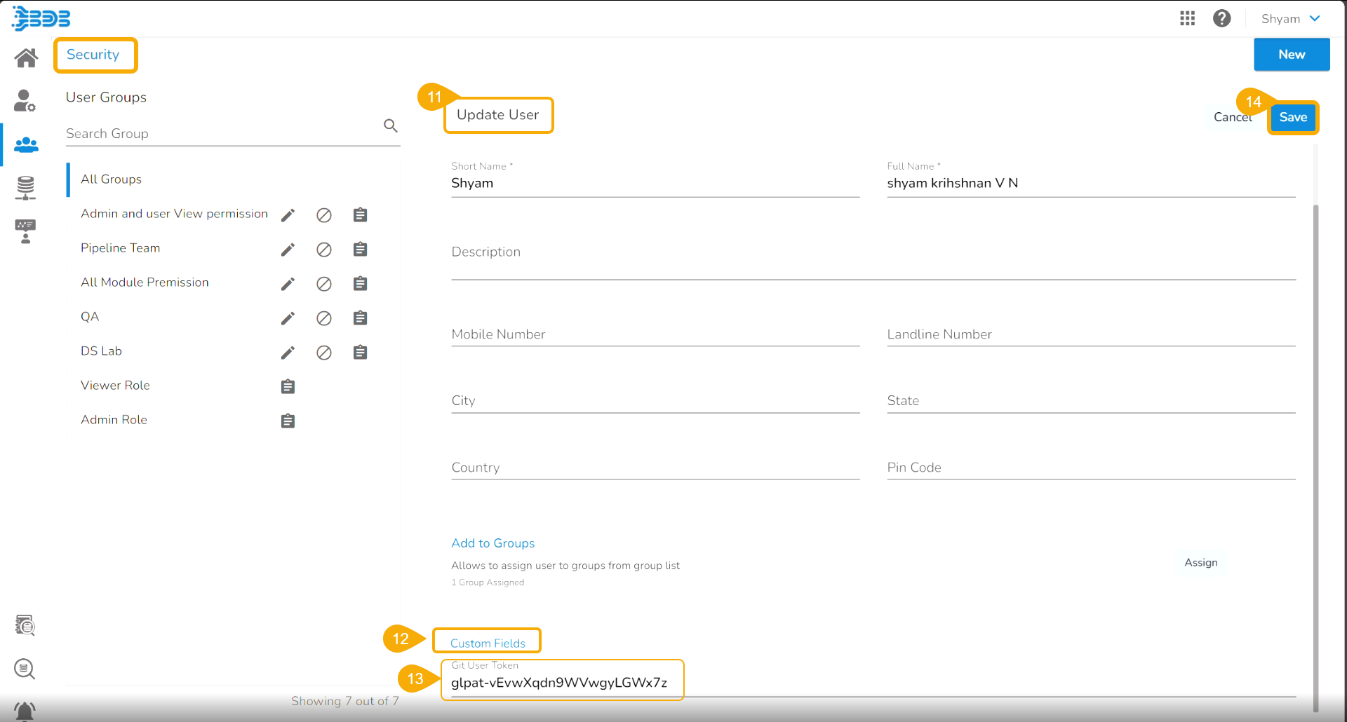
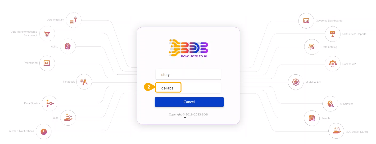
Check out the given walk-through to understand the import of a Migrated DSL Model. inside another user under a different space.
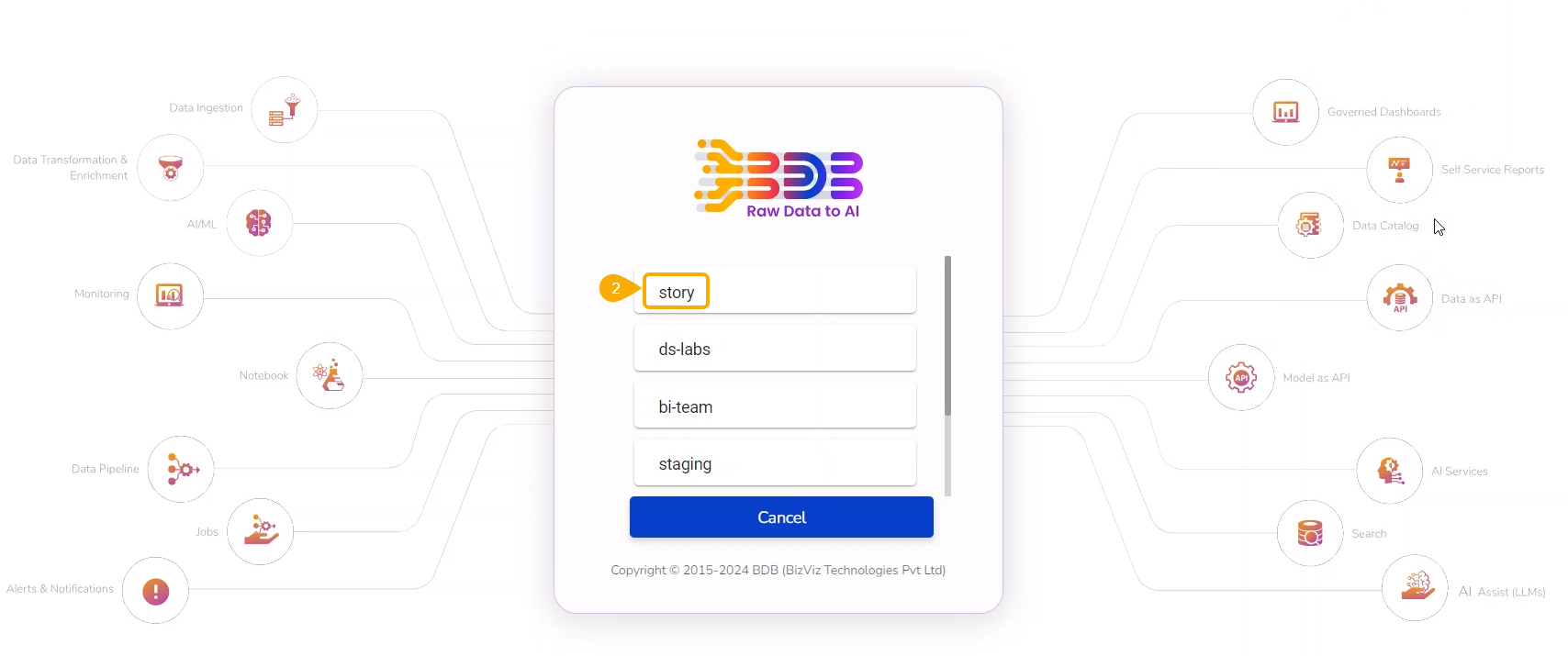
Choose a different user or another space for the same user to import the exported model. In this case, the selected space is different from the space from where the model is exported.
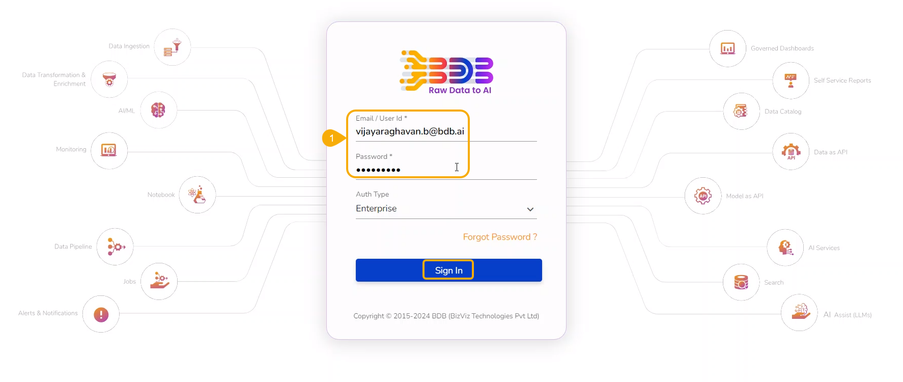
Select a different tenant to sign in to the Platform.
Choose a different space while signing into the platform.
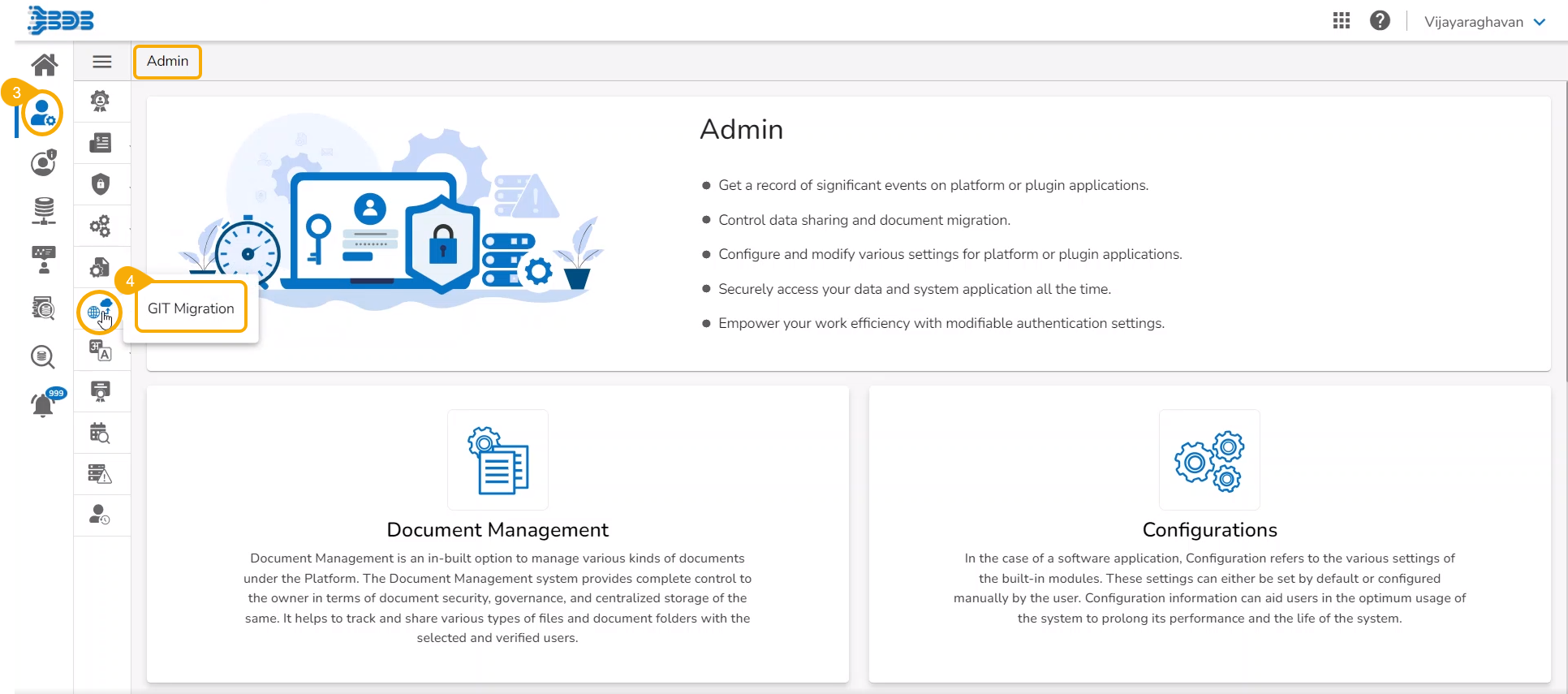
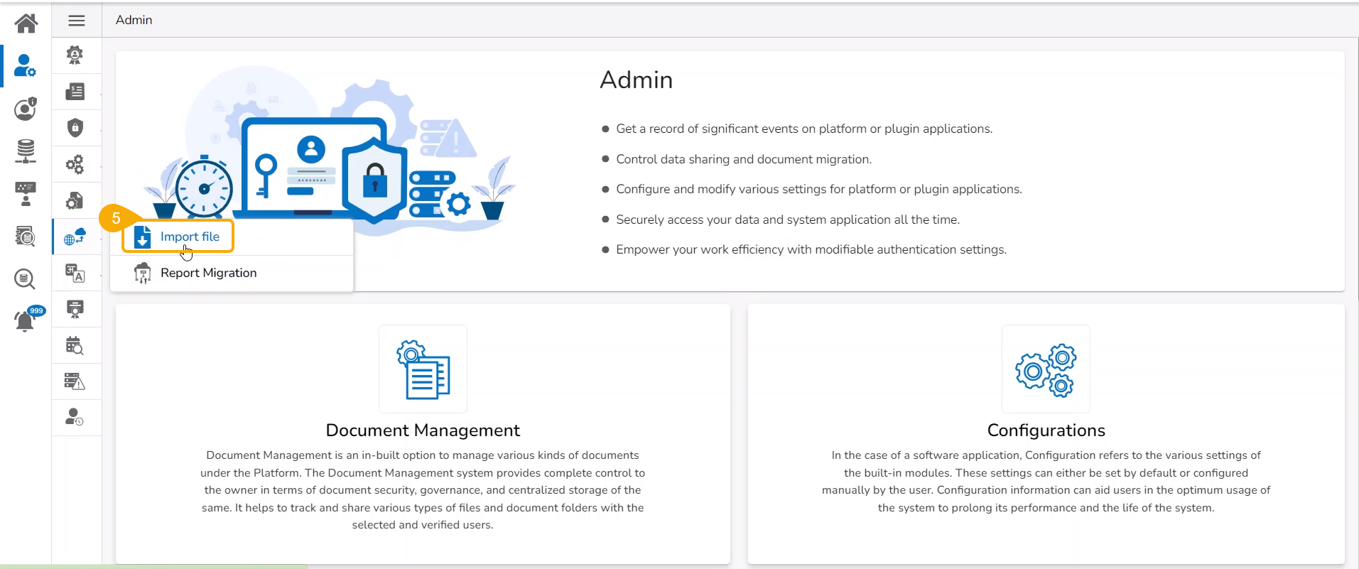
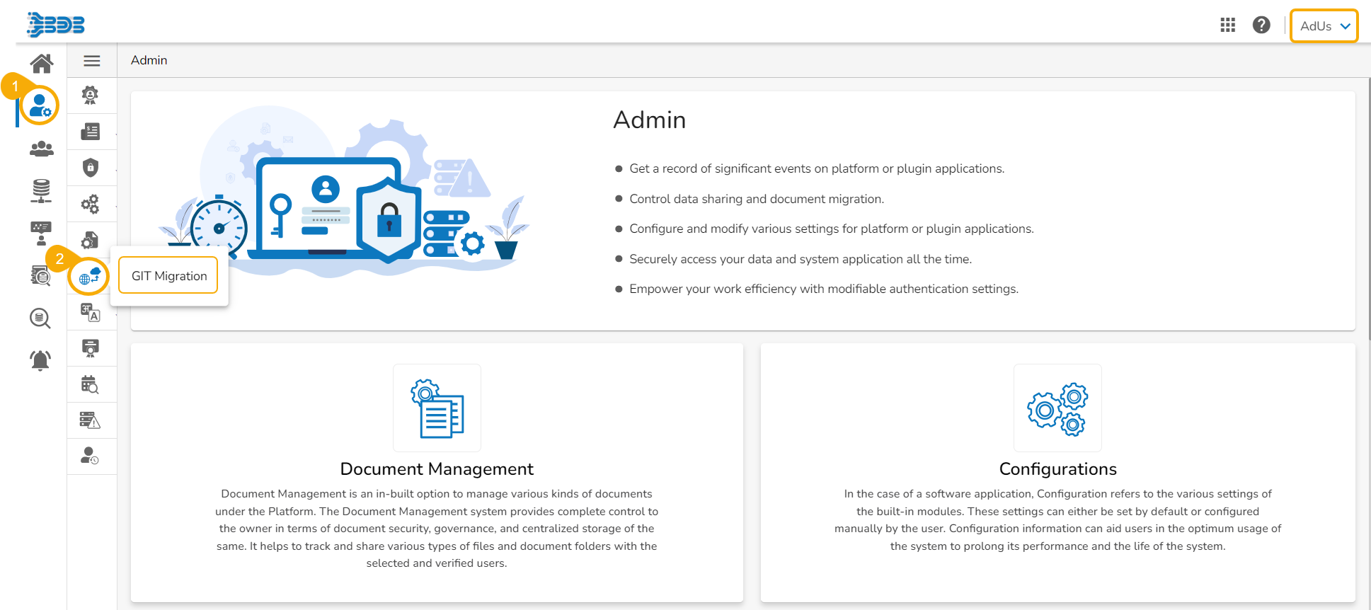
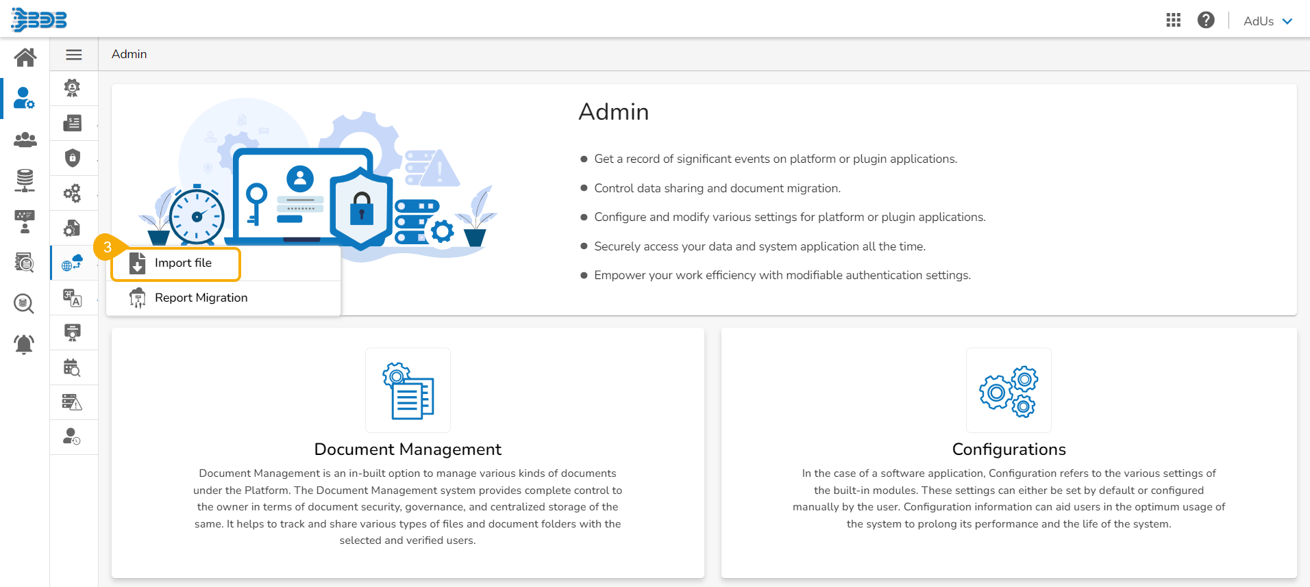
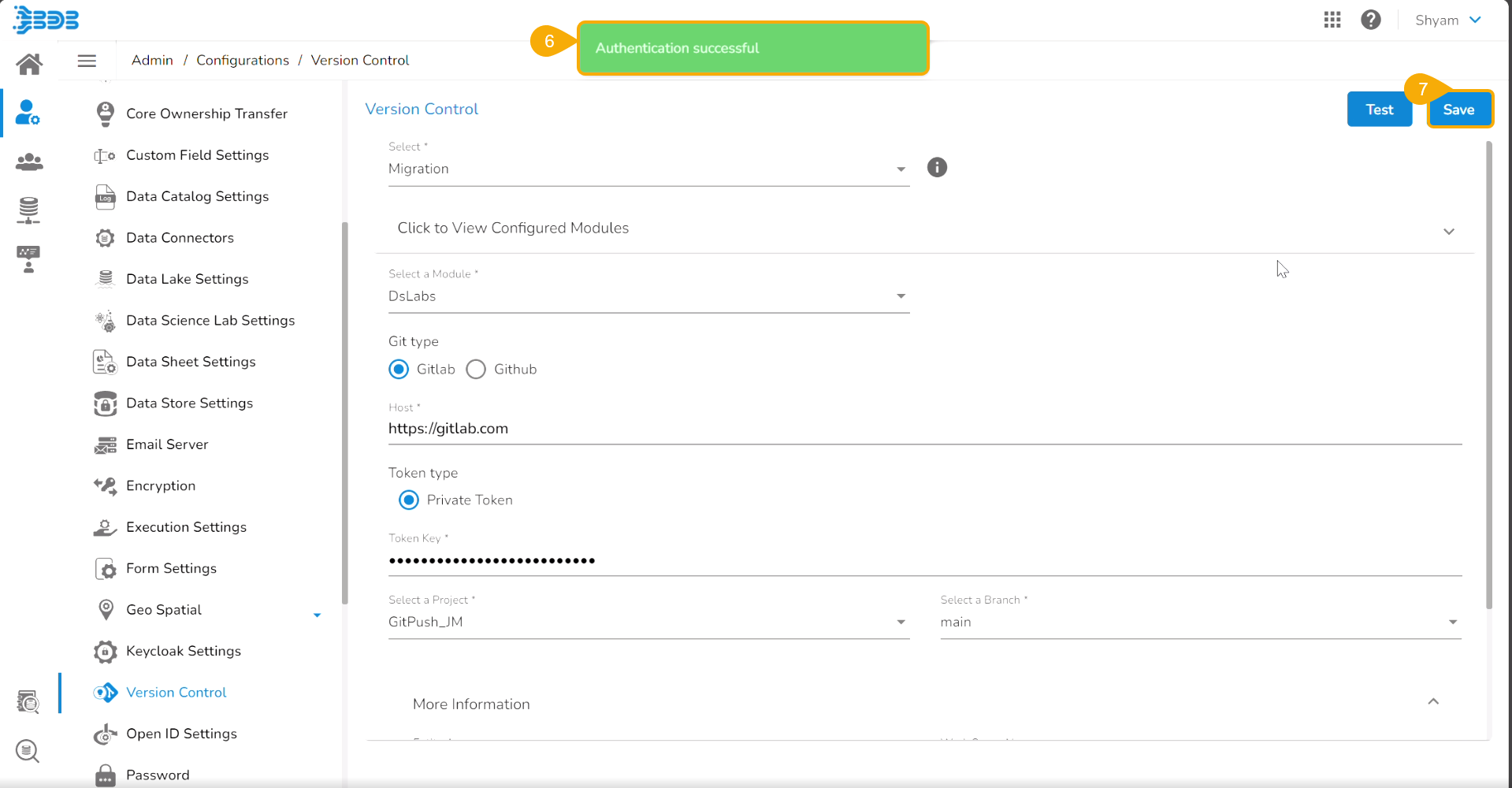
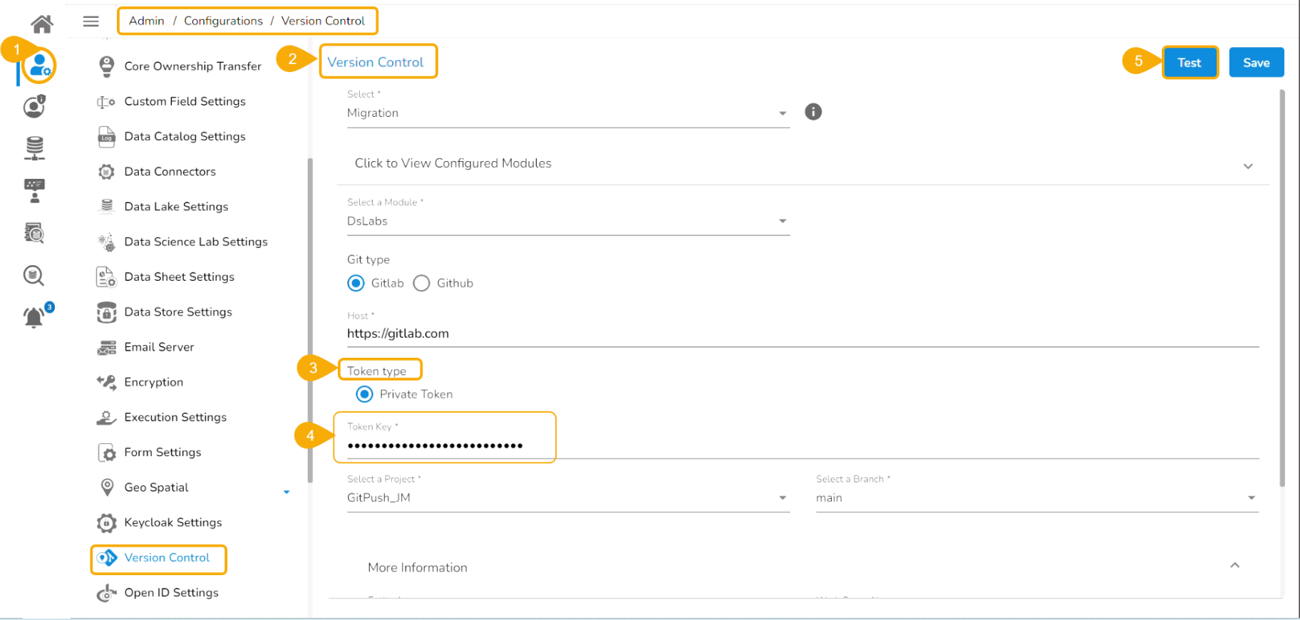
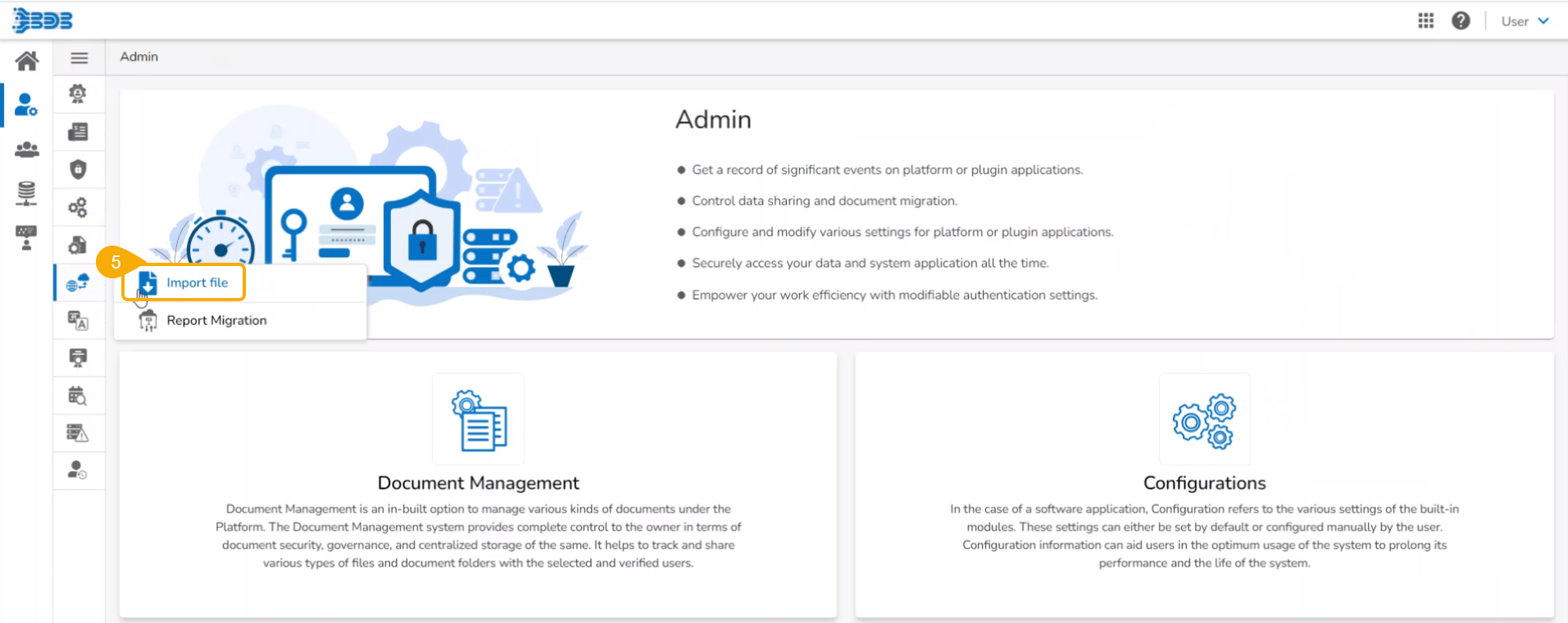
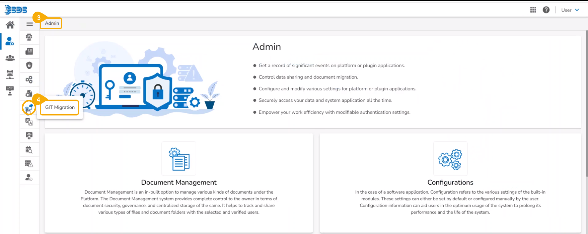
Navigate to the Admin module.
Select the GIT Migration option from the admin menu panel.
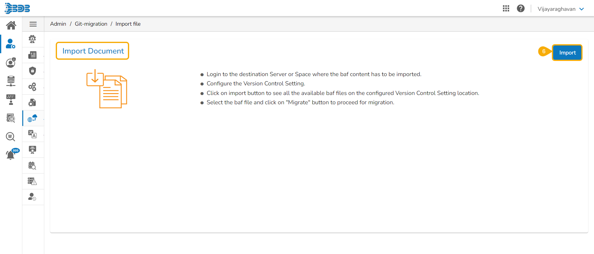
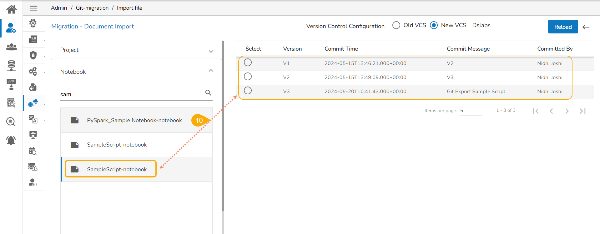
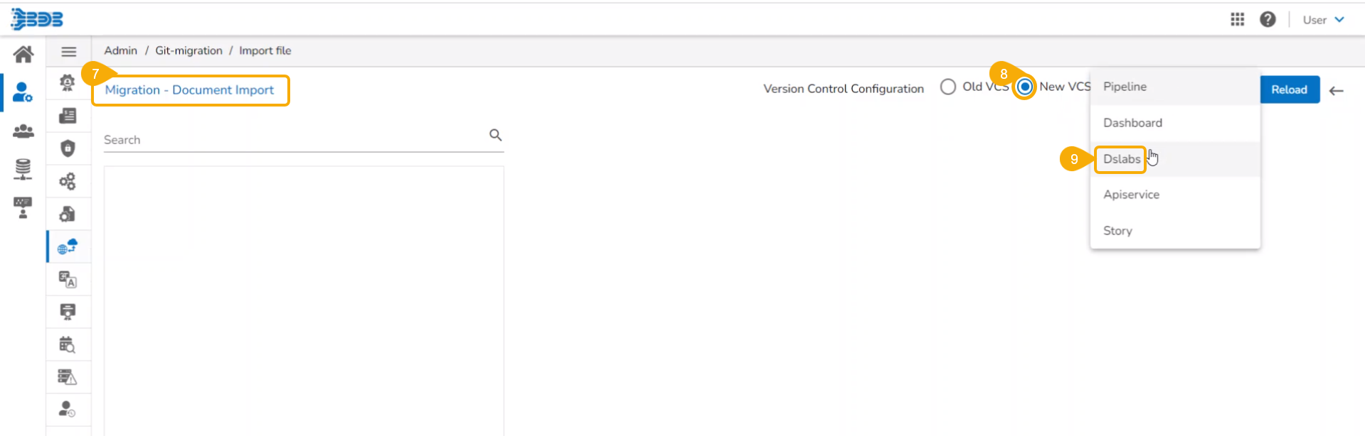
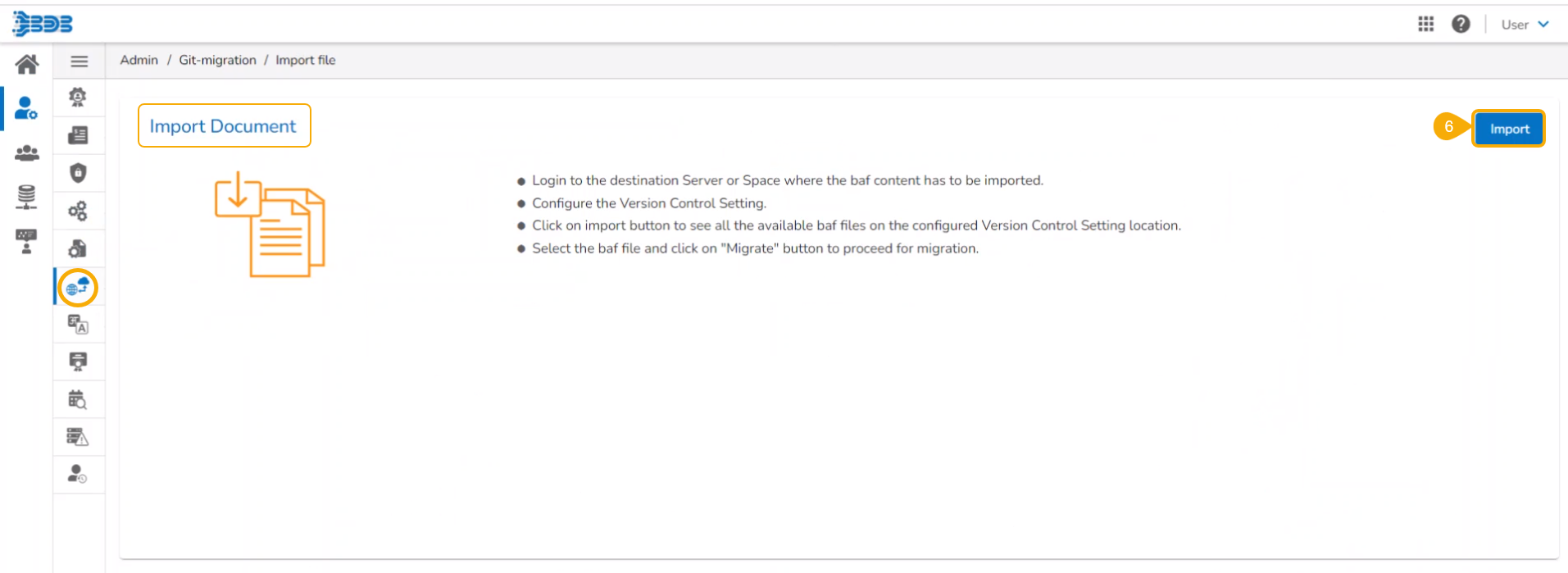
Click the Import File option.
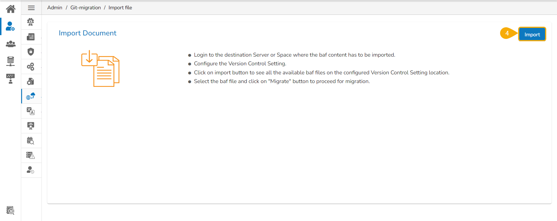
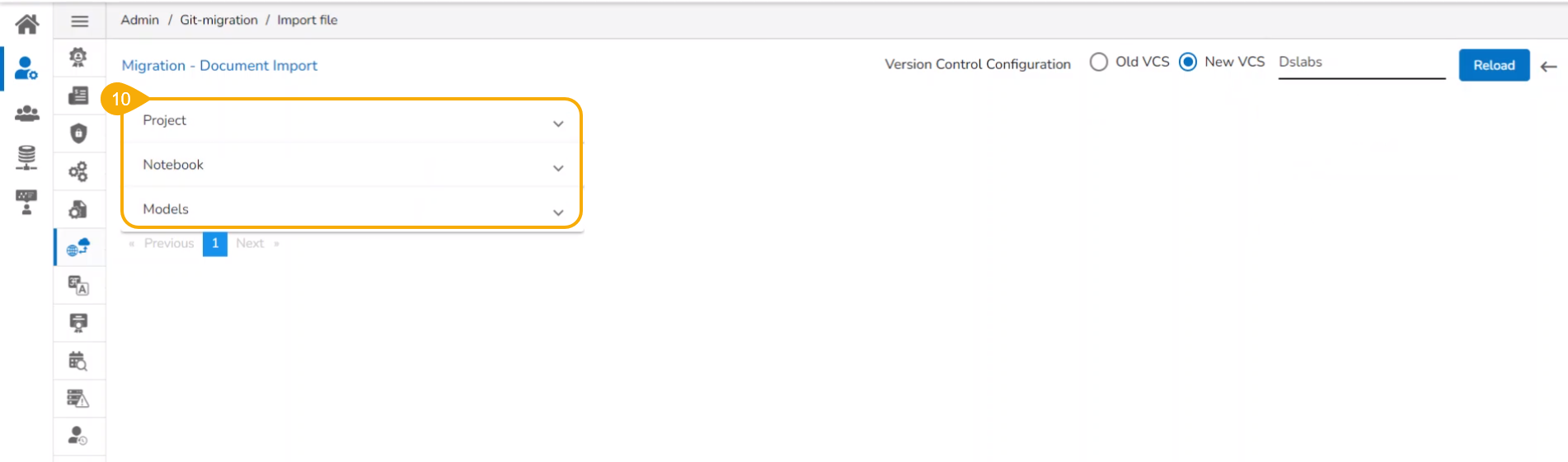
The Import Document page opens, click the Import option.
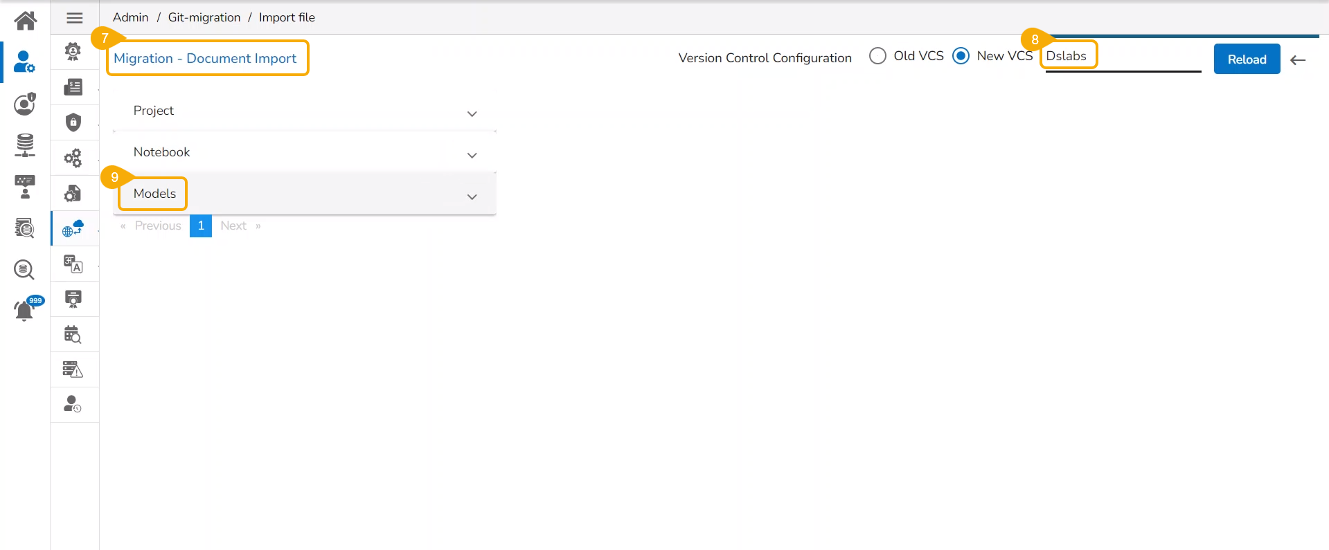
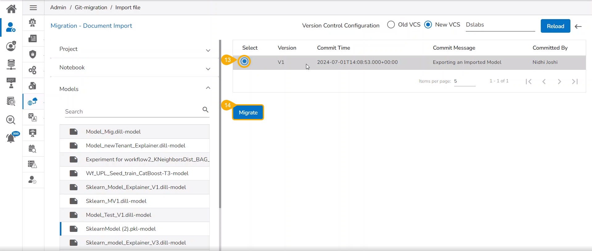
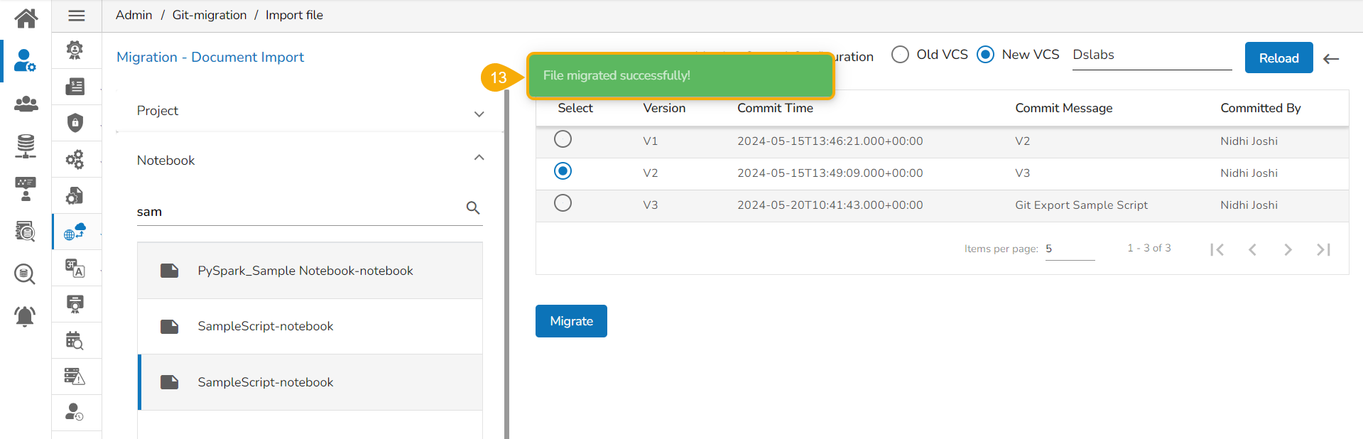
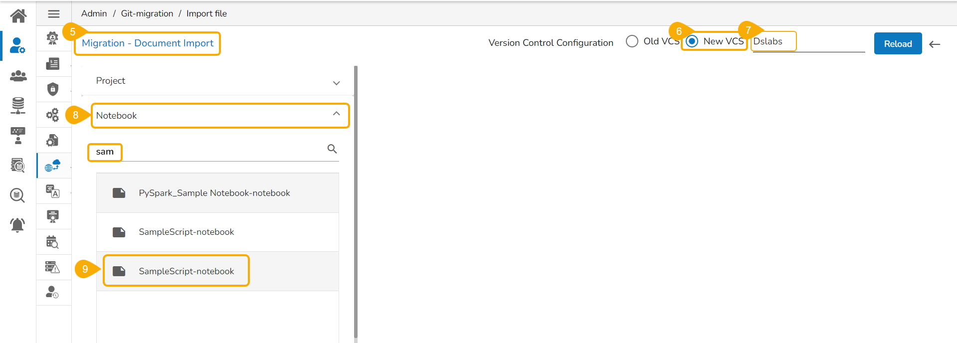
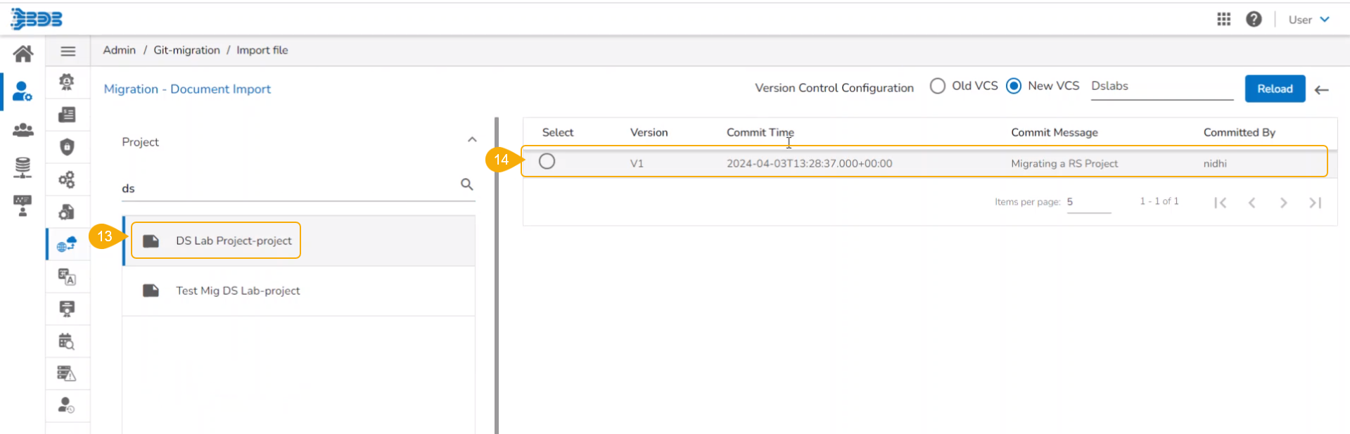
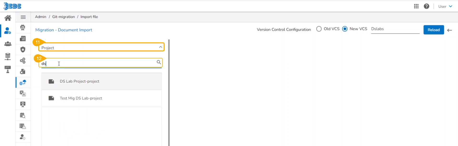
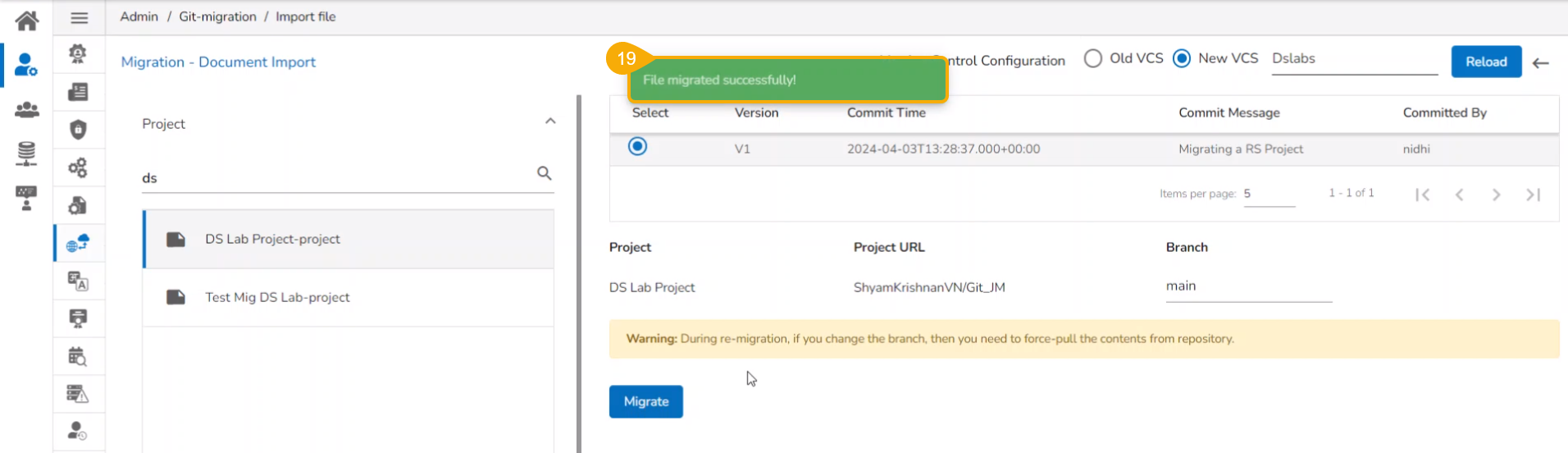
The Migration- Document Import page opens. By default, the New VCS as Version Control Configuration will be selected .
Select the DSLab option from the module drop-down menu.
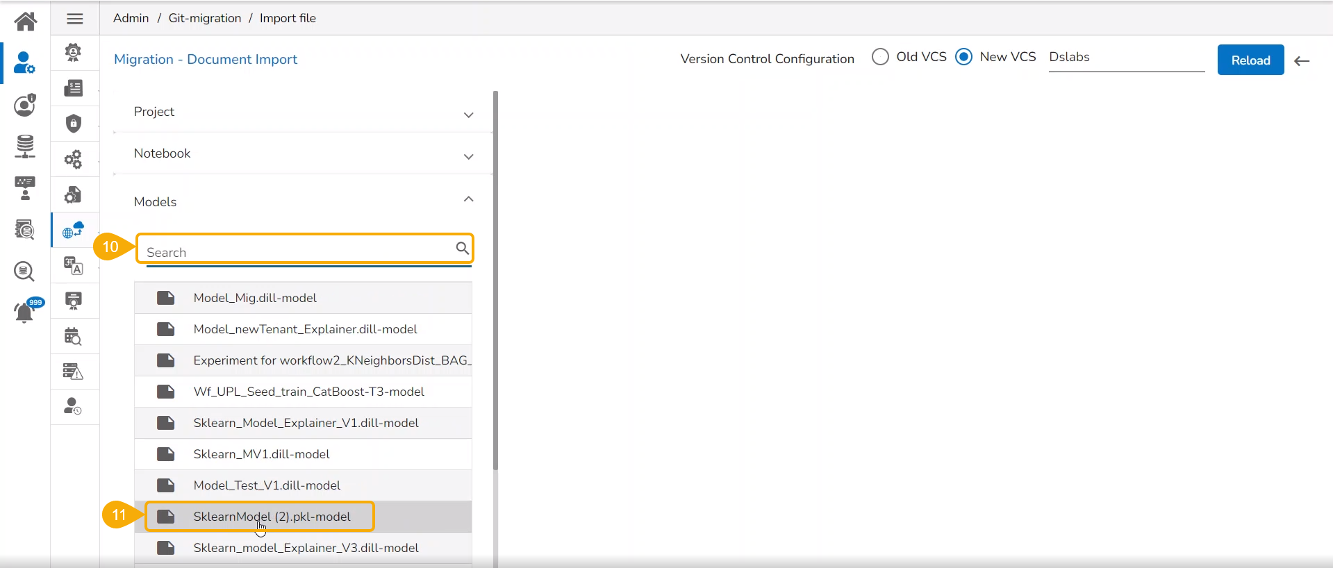
Select the Models option from the left side panel.
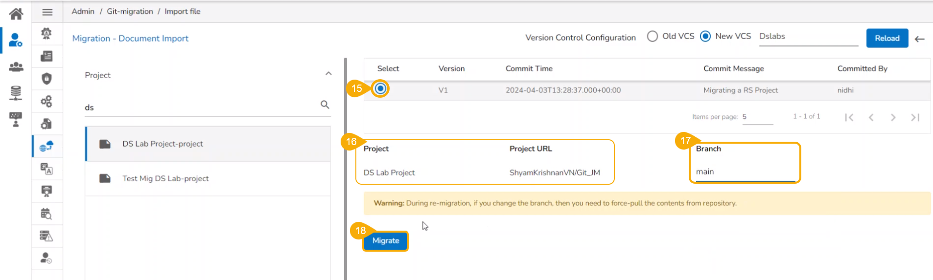
Use Search space to search for a specific model name.
All the migrated Models get listed based on your search.
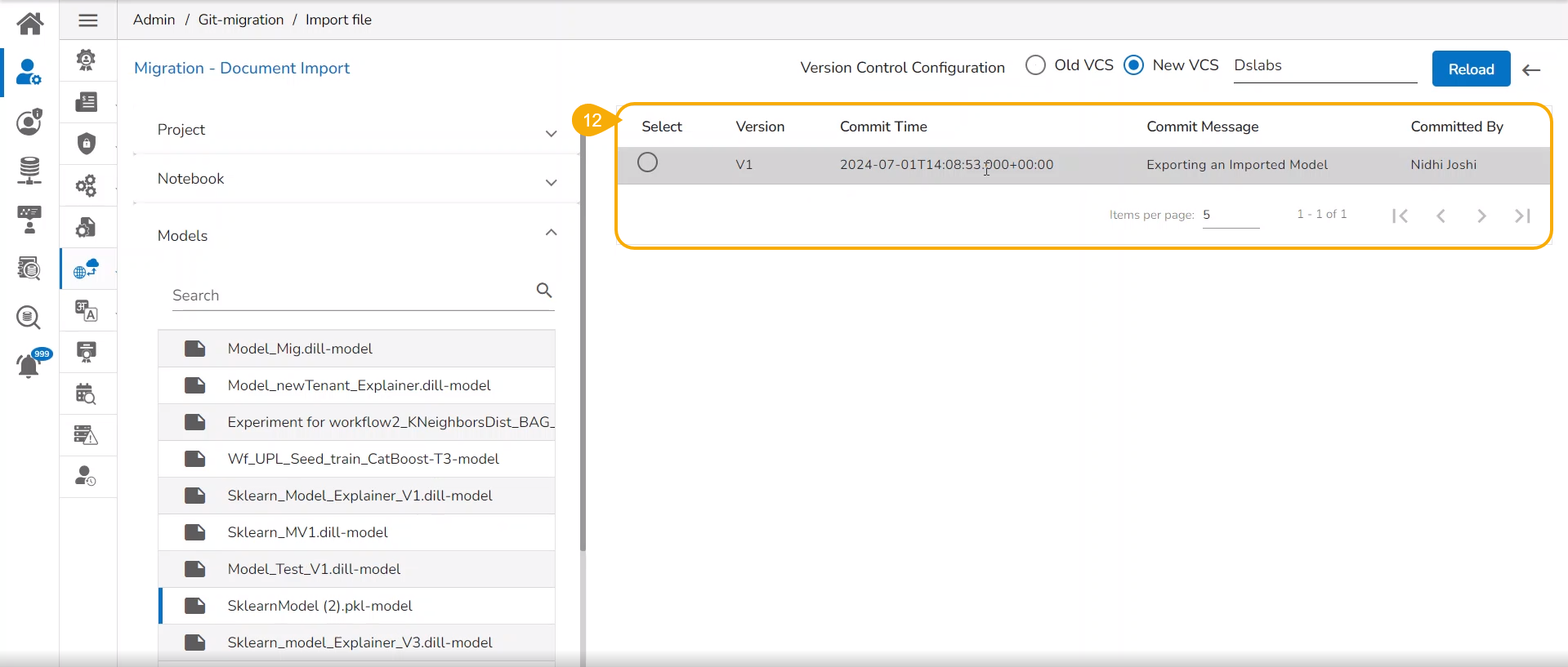
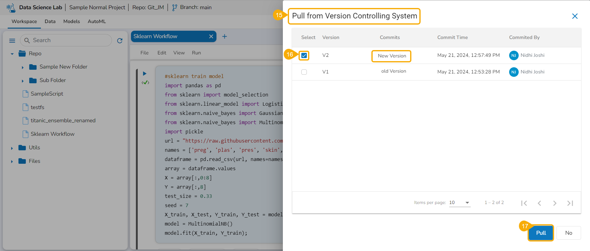
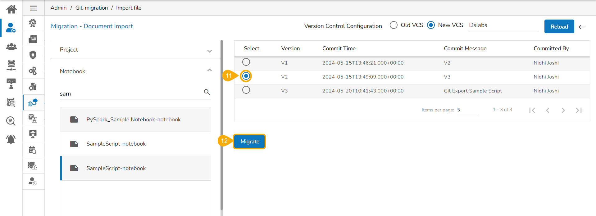
Select a Model from the displayed list to get the available versions of that Model.
Select a Version that you wish to import.
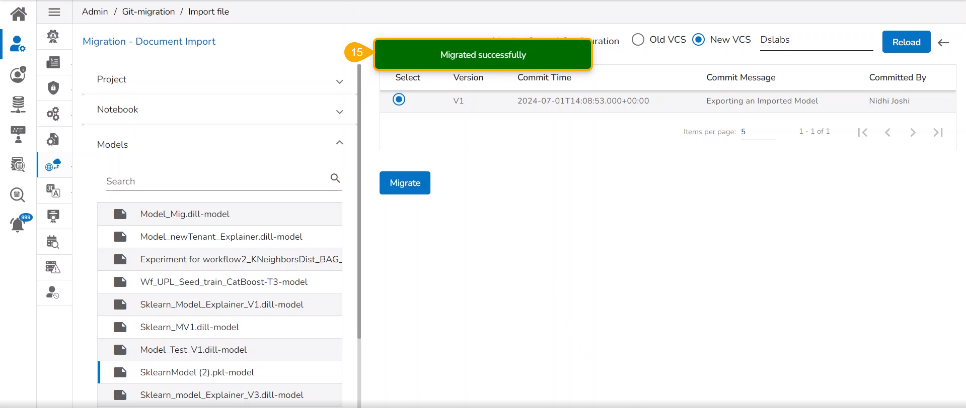
Click the Migrate option.
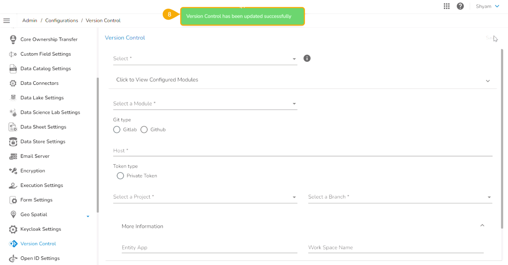
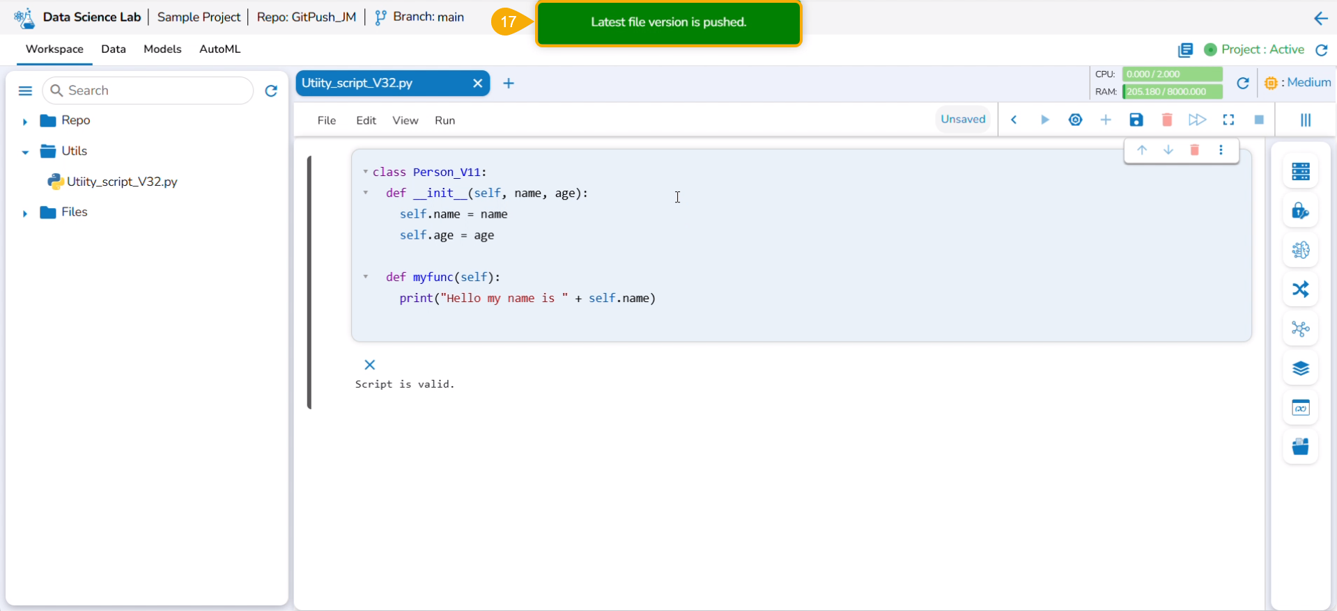
A notification message appears informing that the file has been migrated.
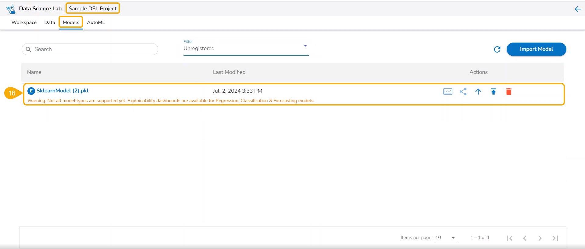
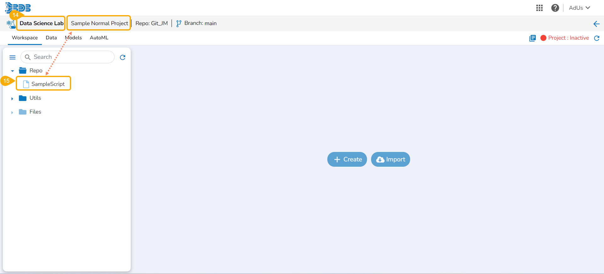
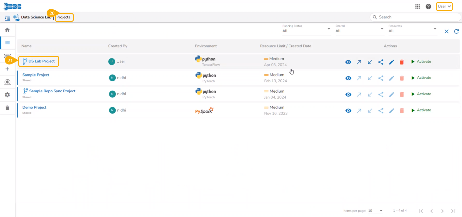
The migrated model gets imported inside the Models tab of the targeted user.
Please Note: While migrating the Model the concerned Data Science Project also gets migrated to the targeted user's account.
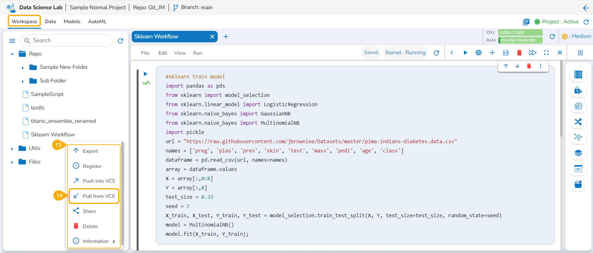
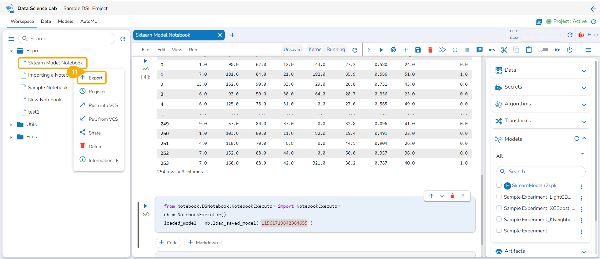
Export
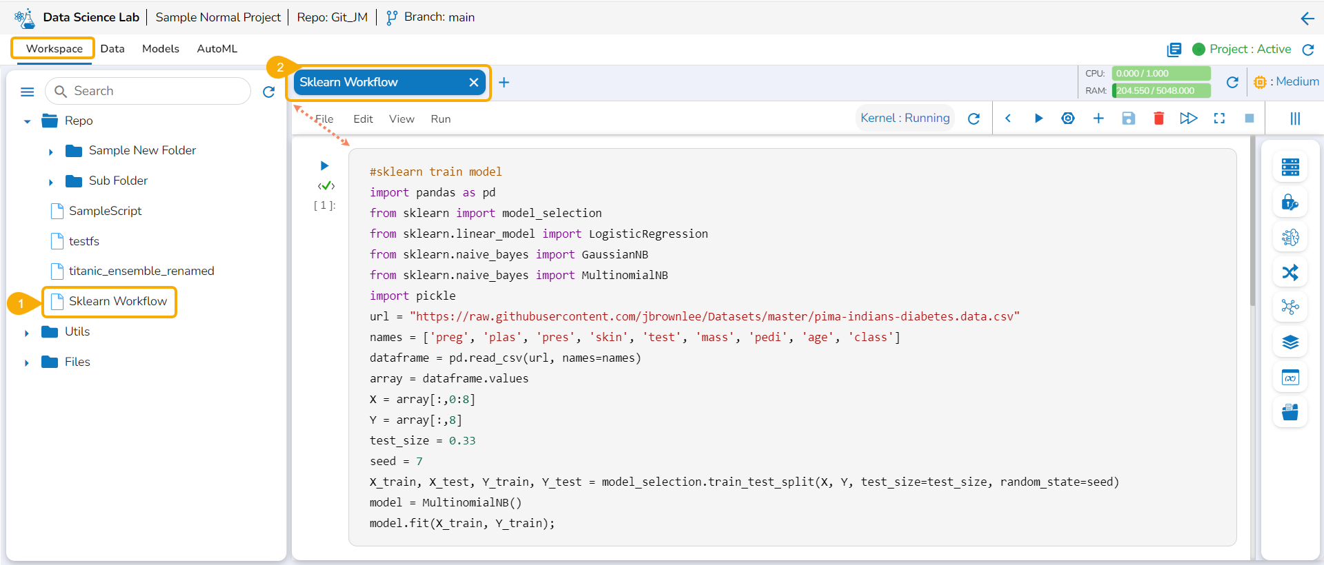
The Export icon provided for a Notebook redirects the user to export the Notebook as a script to the Data Pipeline module and GIT Repository.
Exporting a Data Science Script
A Notebook can be exported to the Data Pipeline module using this option.
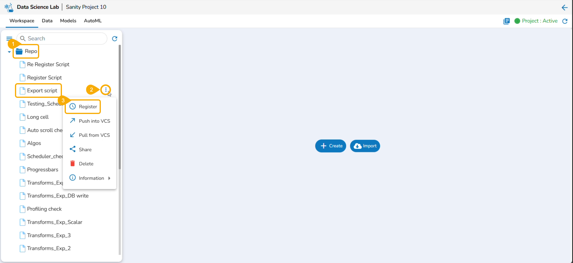
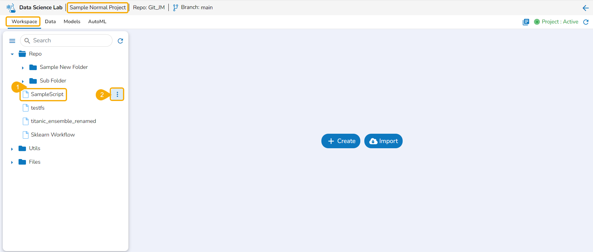
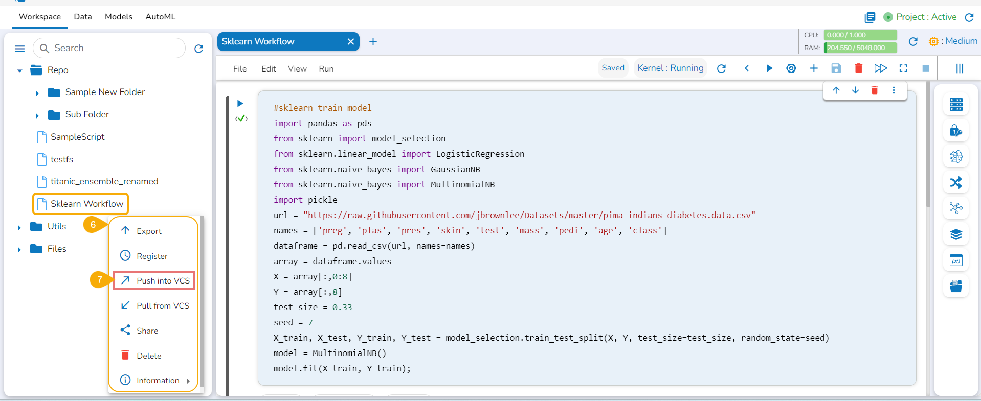
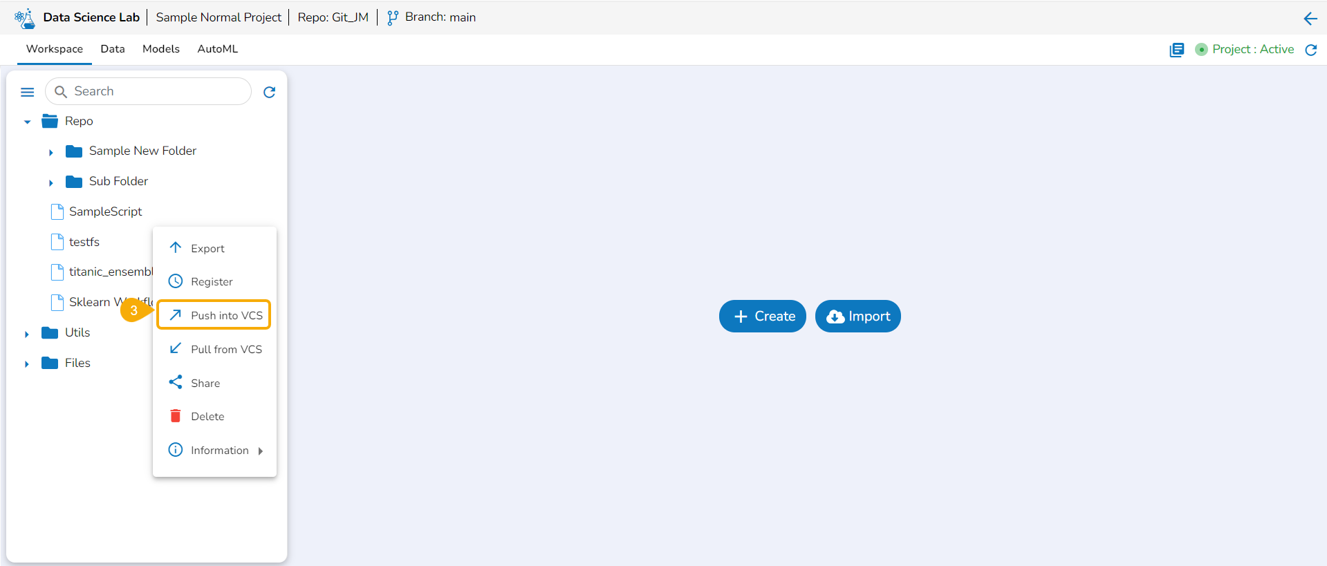
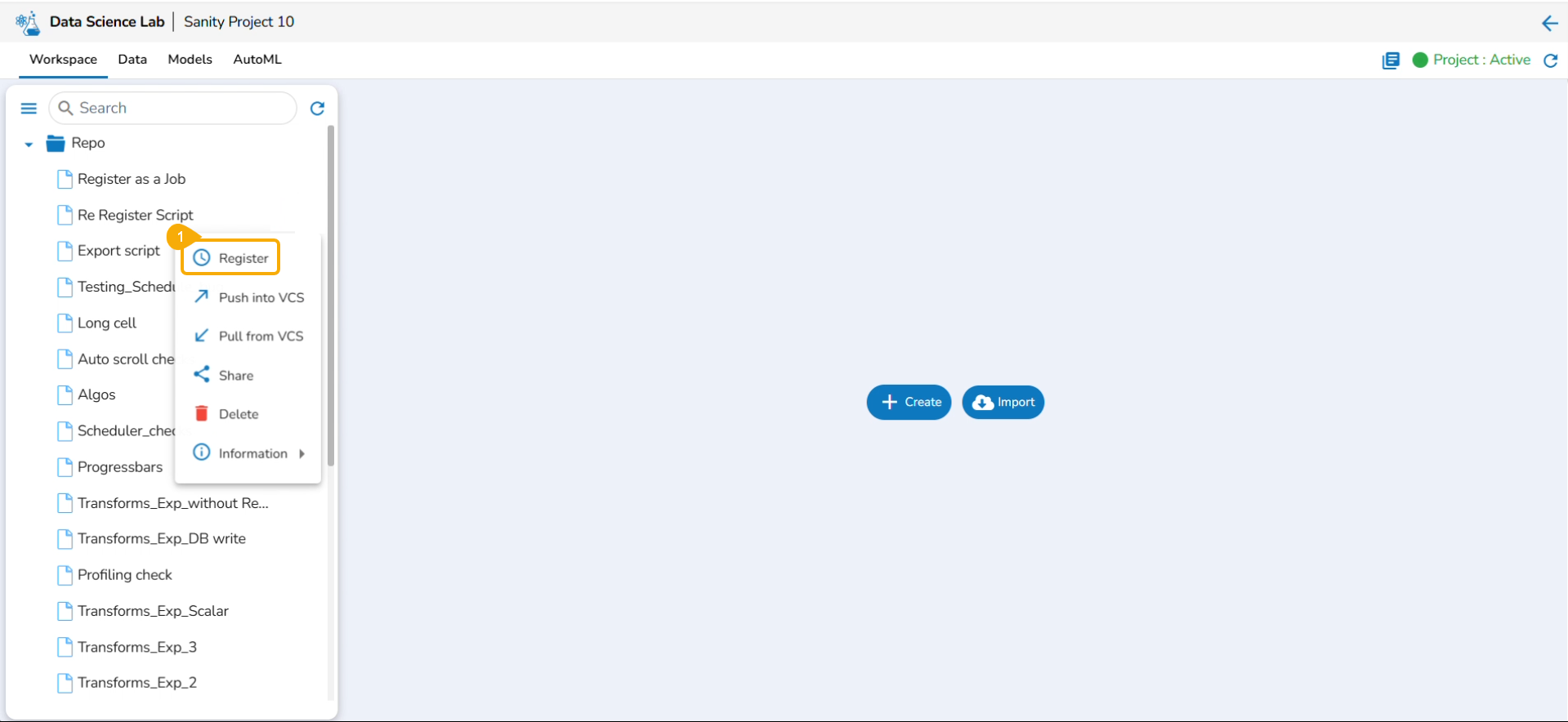
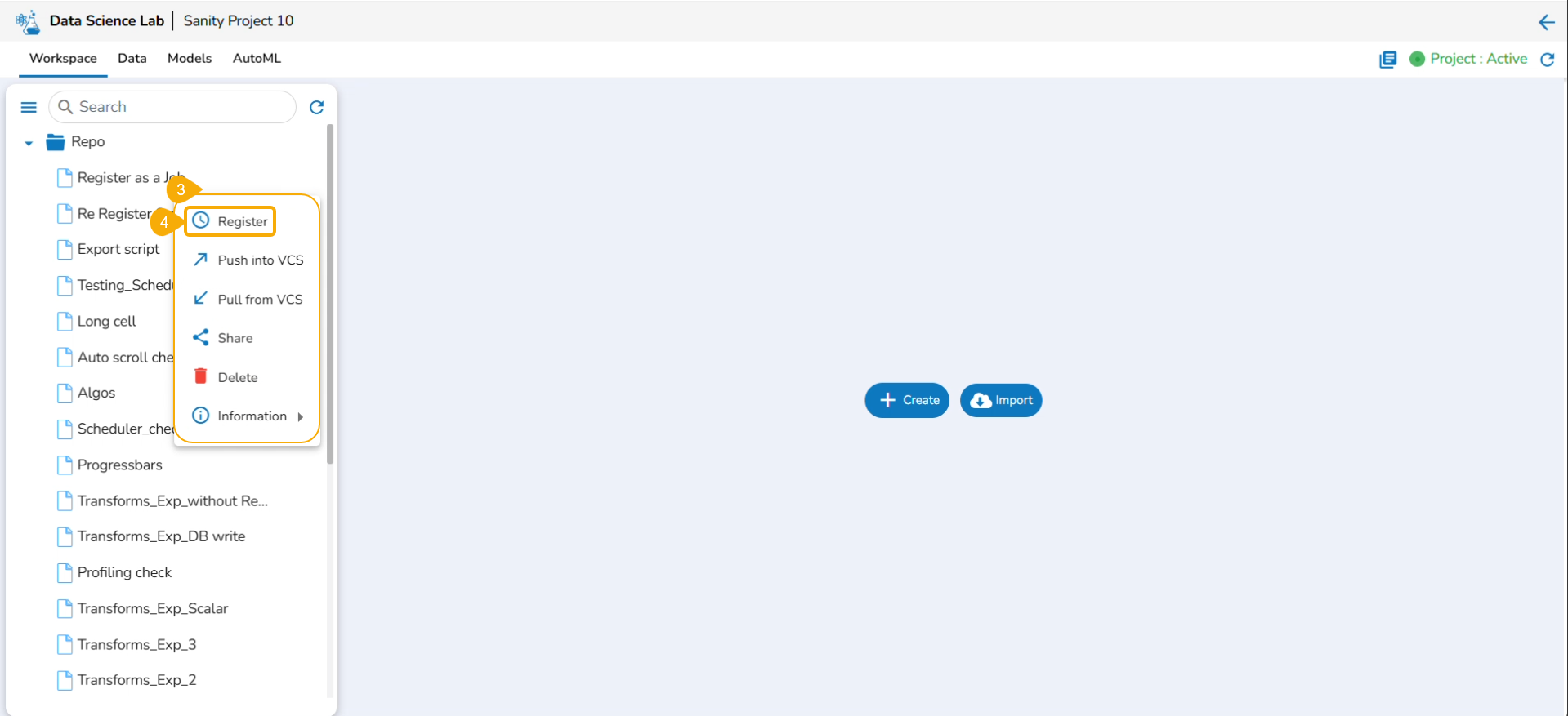
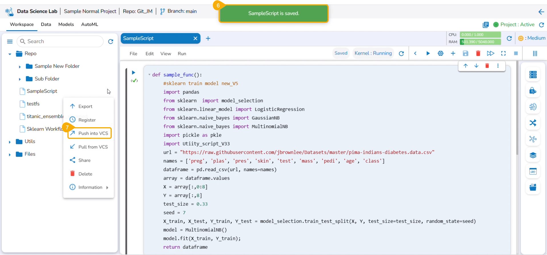
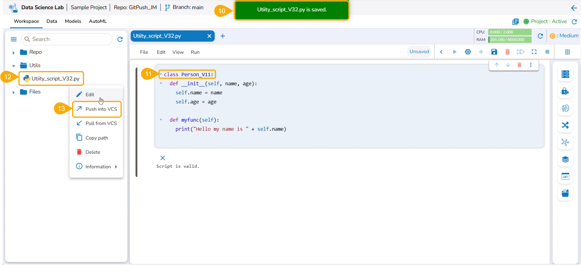
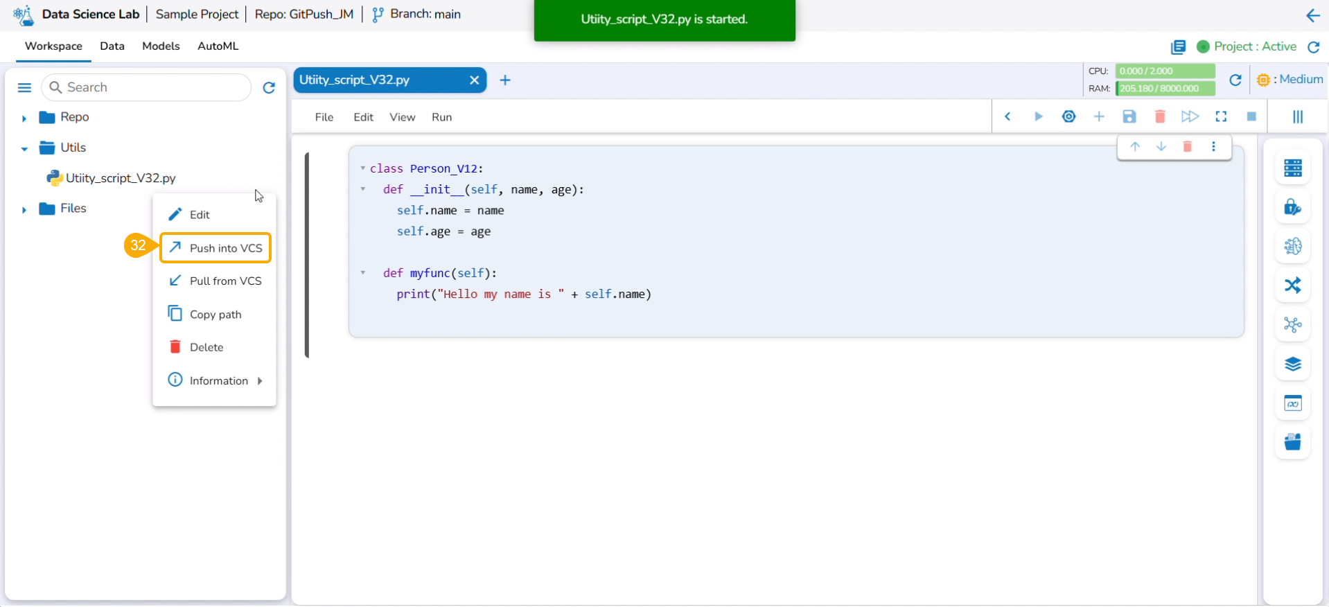
Navigate to the Repo folderand select a Notebook from the Workspace tab.
Click the Ellipsis icon for the selected Notebook to open the context menu.
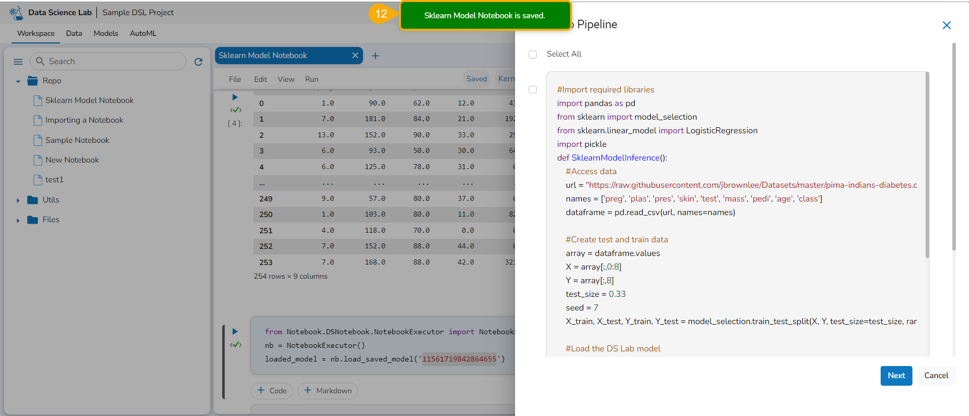
Click the Register option for the Notebook.
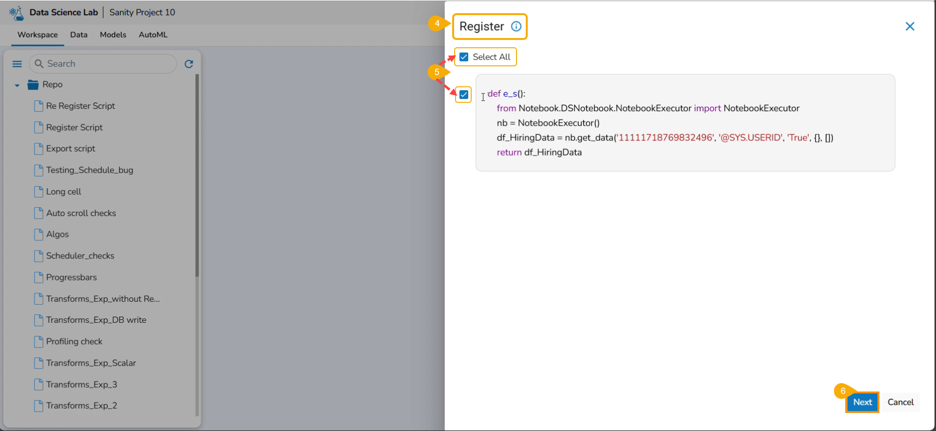
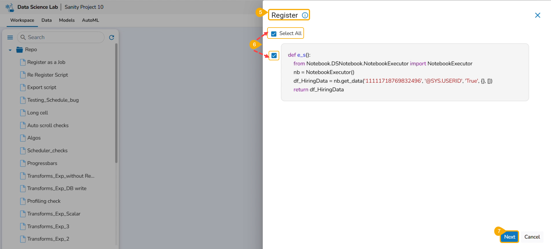
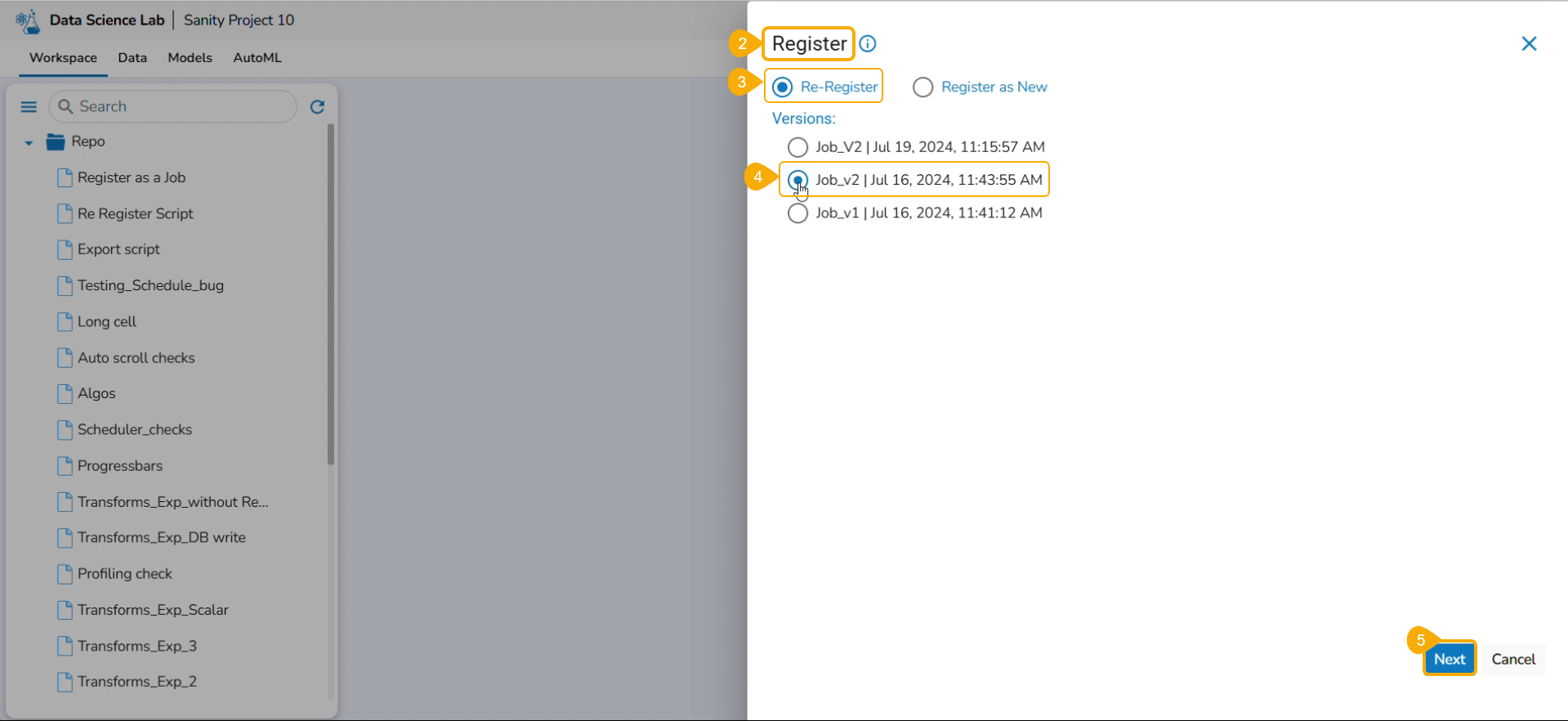
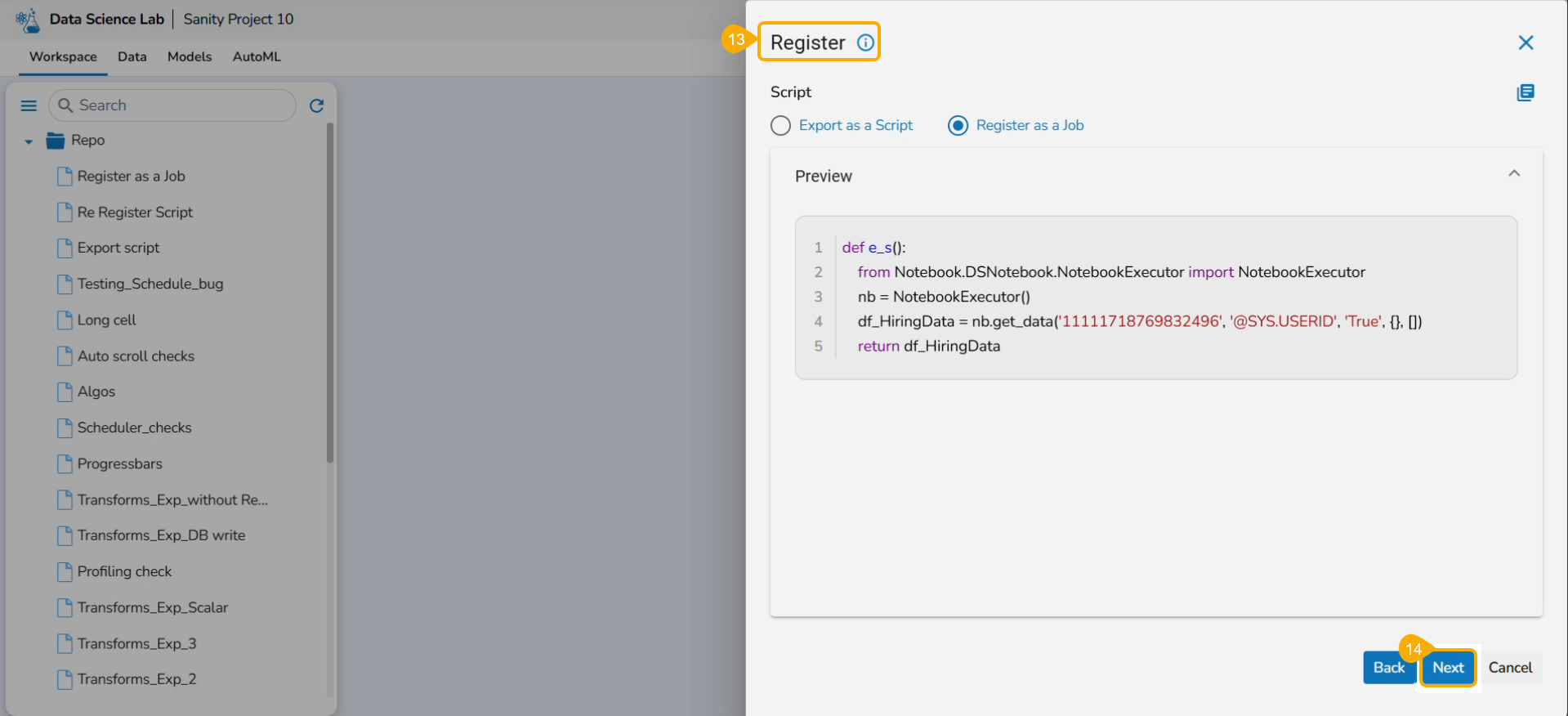
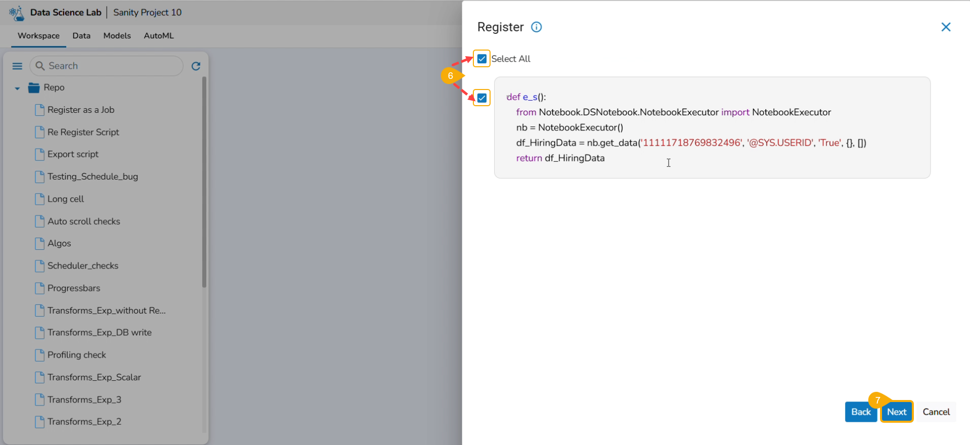
The Register windowopens.
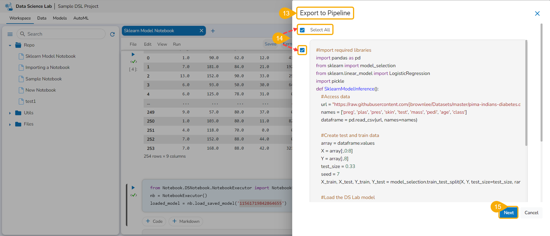
Select the Select All option or the required script using the checkbox(es).
Click the Next option.
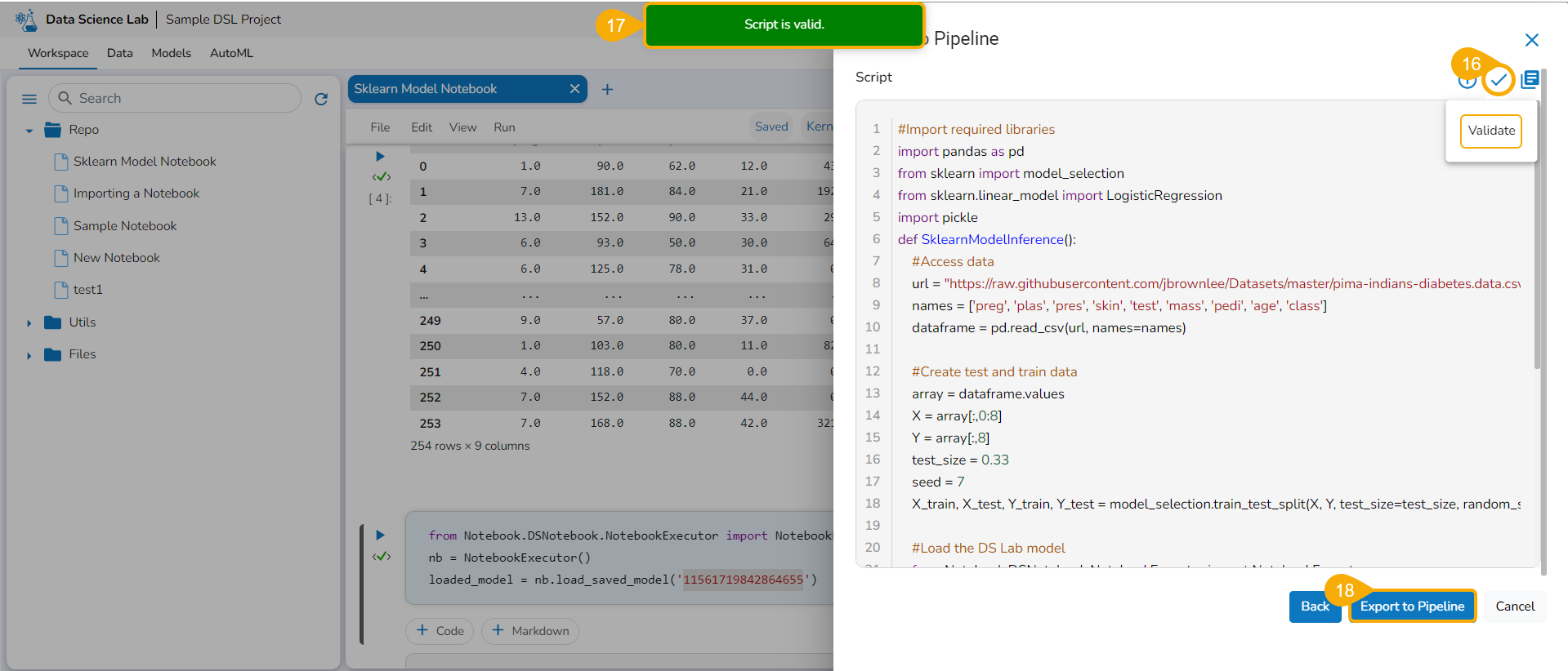
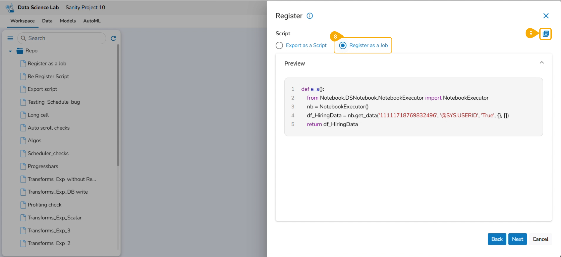
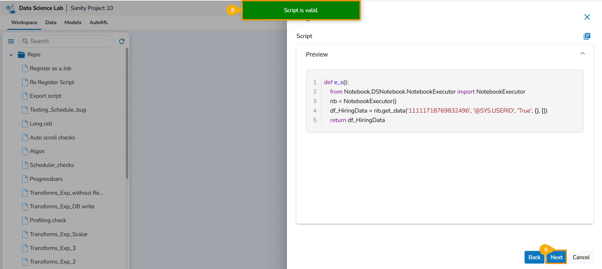
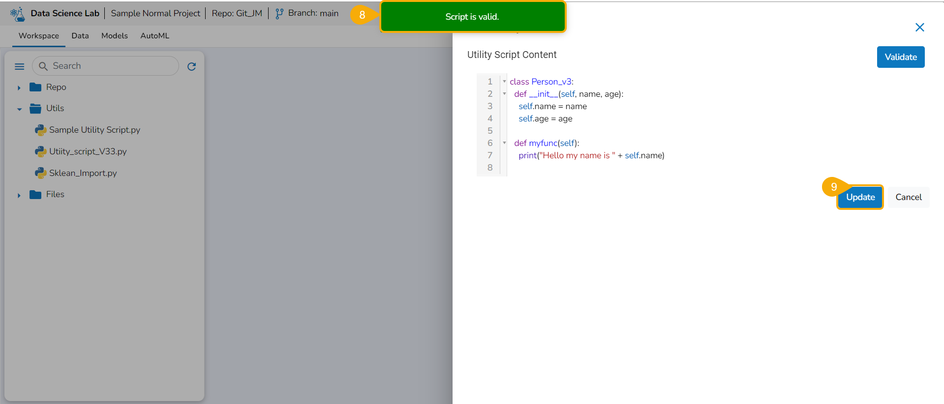
Please Note: The user must write a function to use the Export to Pipeline functionality.
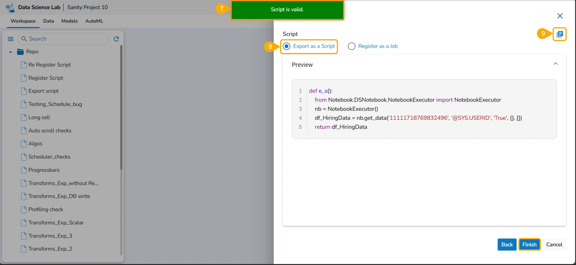
A notification appears stating that the selected script is valid.
Select Export as a Script option by selecting it via the checkbox.
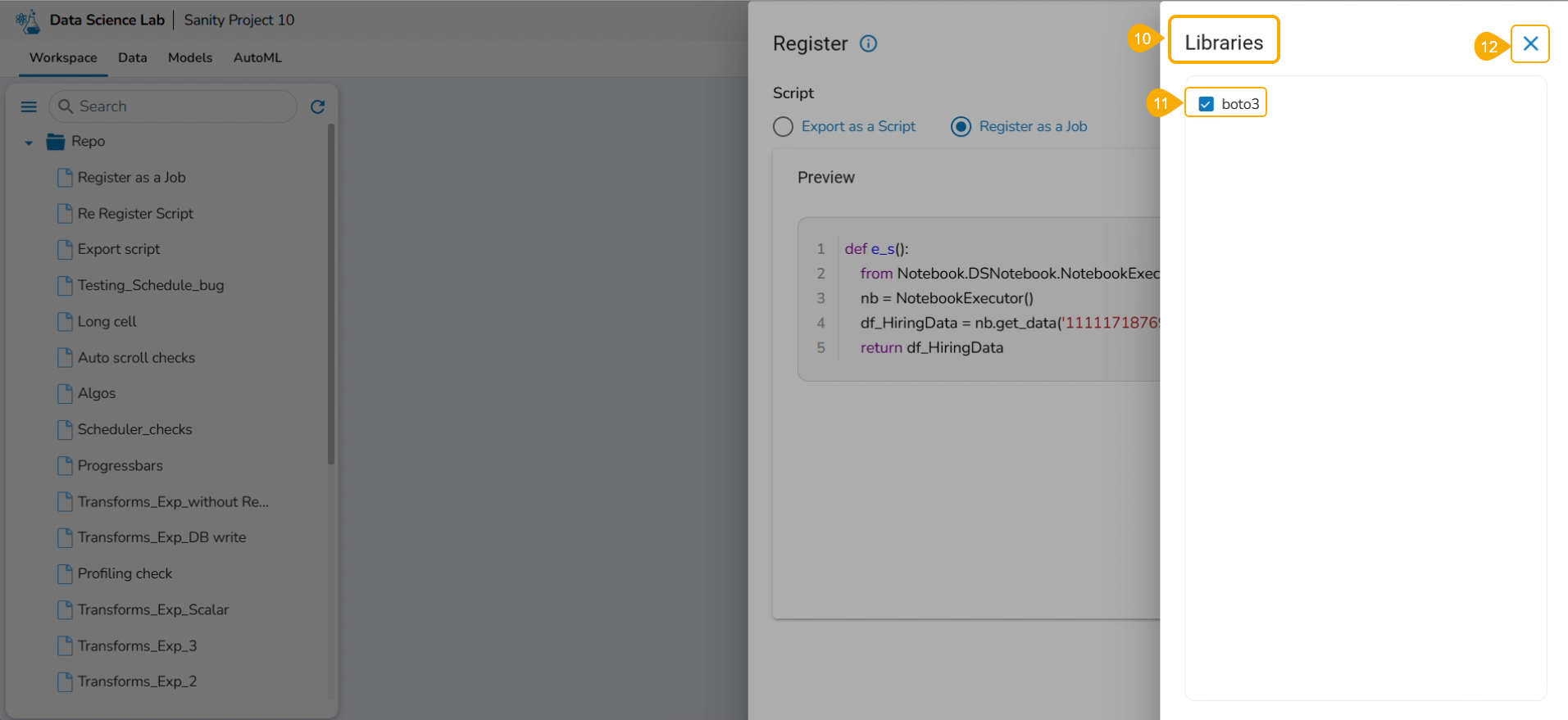
Click the Libraries icon.
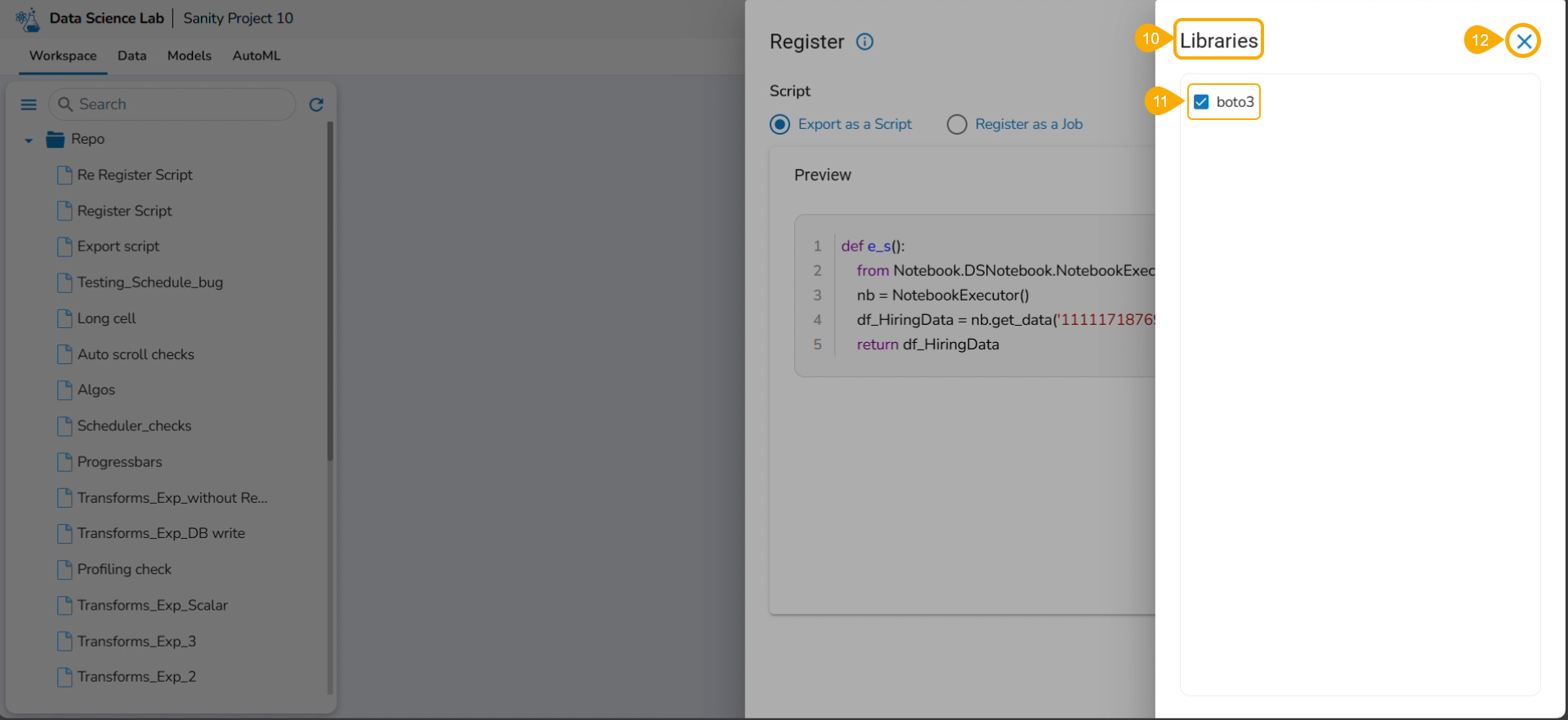
The Libraries drawer opens.
Select available libraries by using checkboxes.
Click the Close icon to close the Libraries drawer.
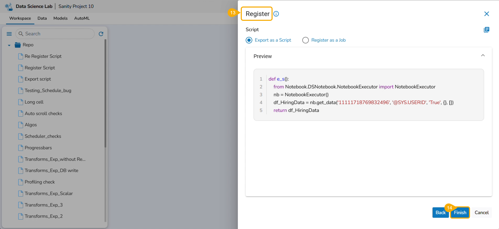
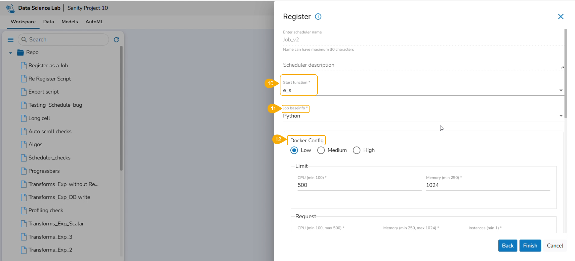
The user gets redirected to the Register page.
Click the Finish option.
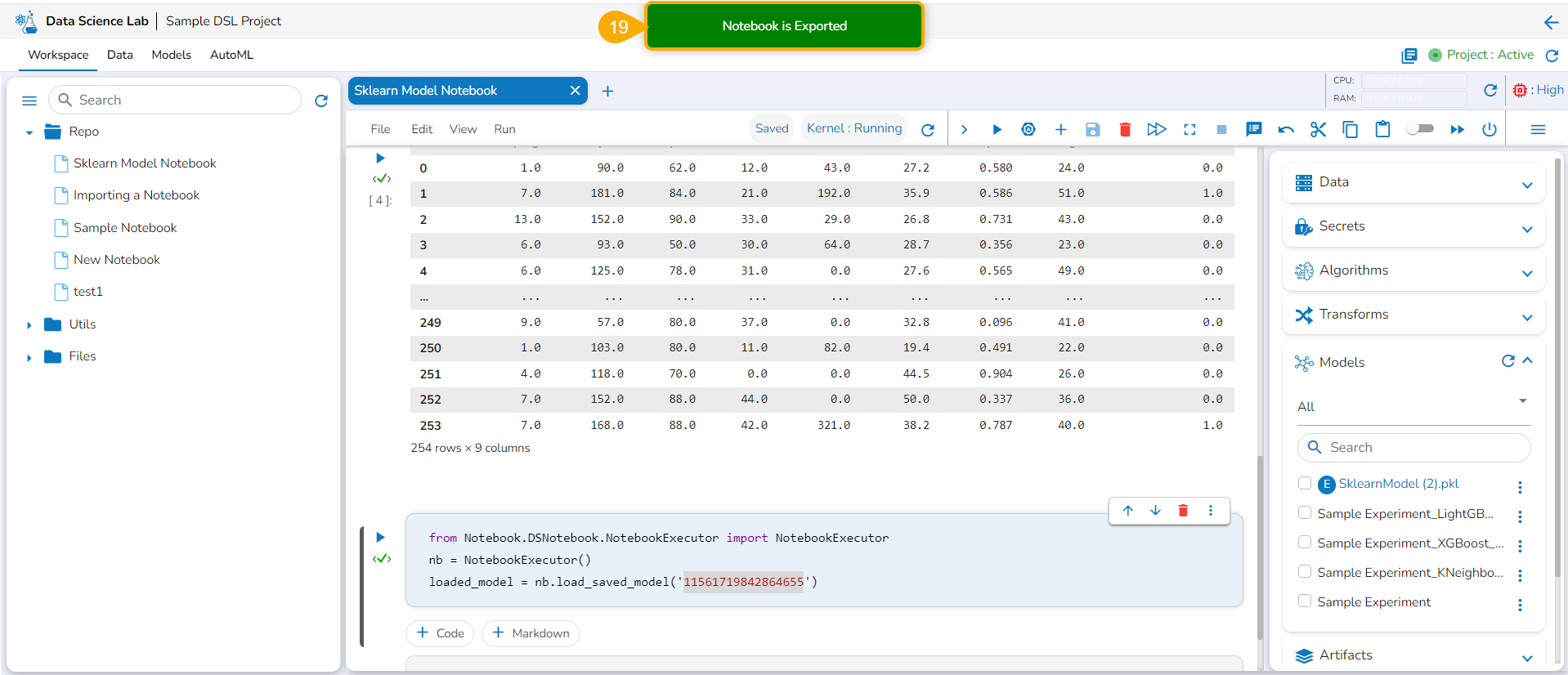
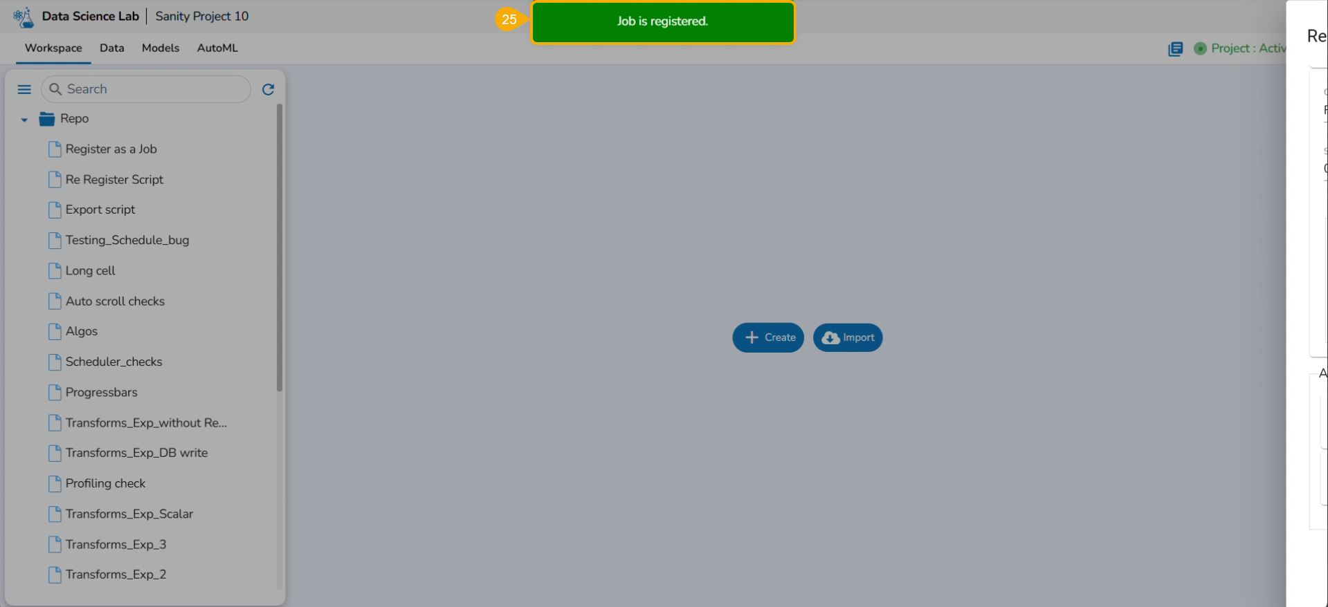
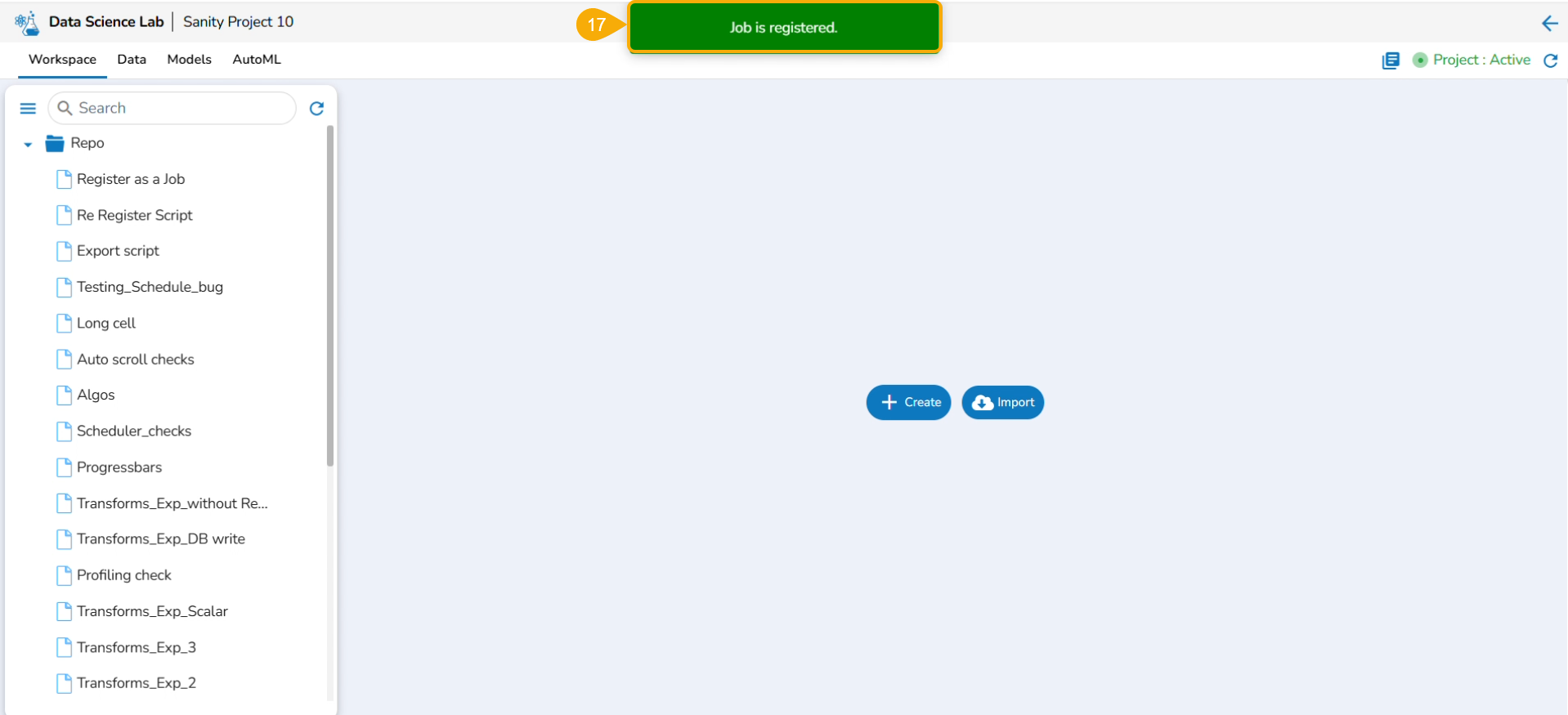
A notification message appears to ensure that the selected script is exported.
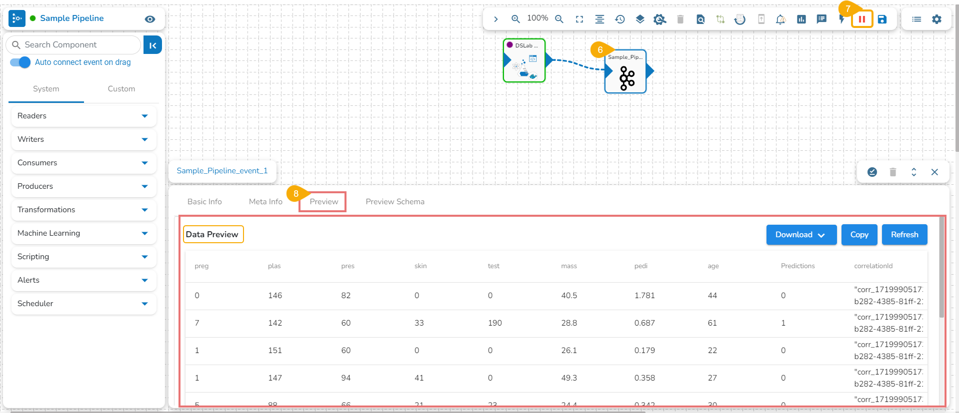
Please Note: The exported script will be available for the Data Pipeline module to be consumed inside a DS Lab Runner component.
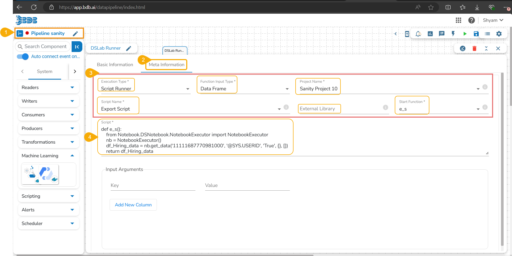
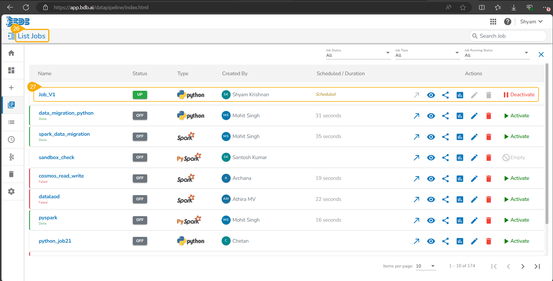
Accessing an Exported Script in the Data Pipeline
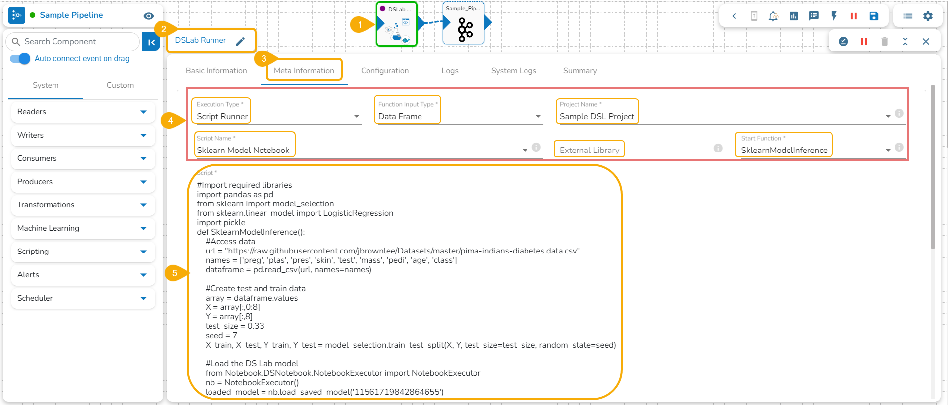
Navigate to a Data Pipeline containing the DS Lab Runner component.
Open the Meta Information tab of the DS Lab Runner component.
Select the required information as given below to access the exported script:
Secrets
Generate Environment Variables to save your confidential information from getting exposed.
You can generate Environment variables for the confidential information of your database using the Secret Management function. Thus, it saves your secret information from getting exposed to all the accessible users.
Pre-requisite:
The users must configure the using the Admin module of the platform before attempting the Secret option inside the DS Lab module.
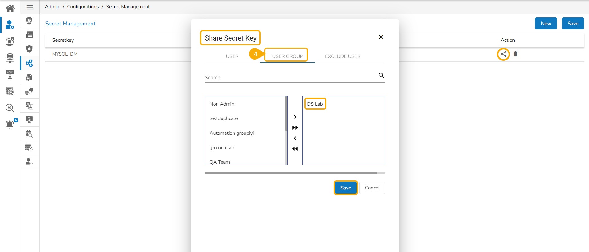
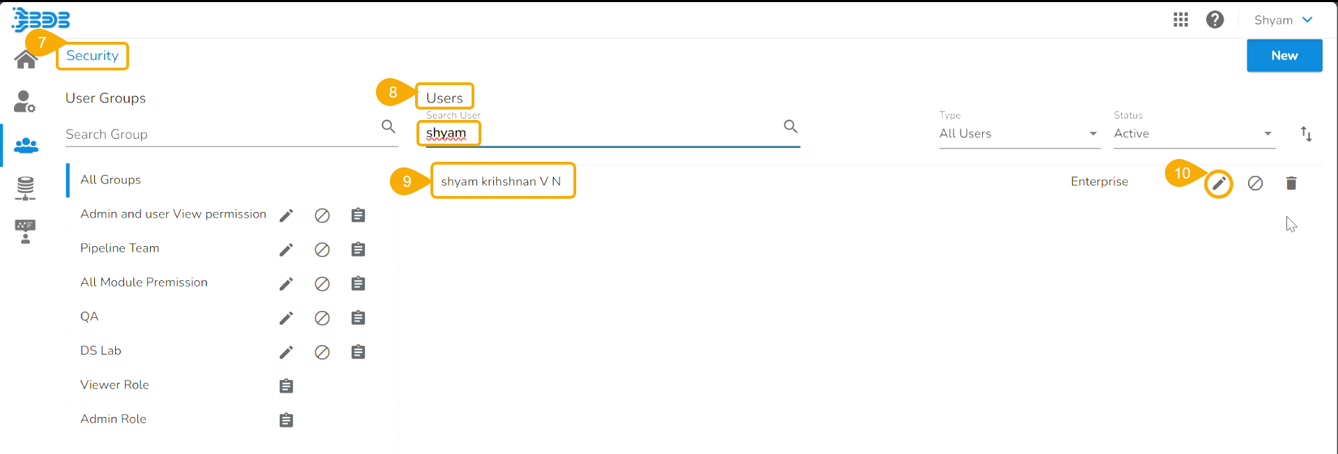
The configured Secrets must be shared with a user group to access it inside the Data Science Lab module.
The user account selected for this activity must belong to the same user group to which the configured secrets were shared.
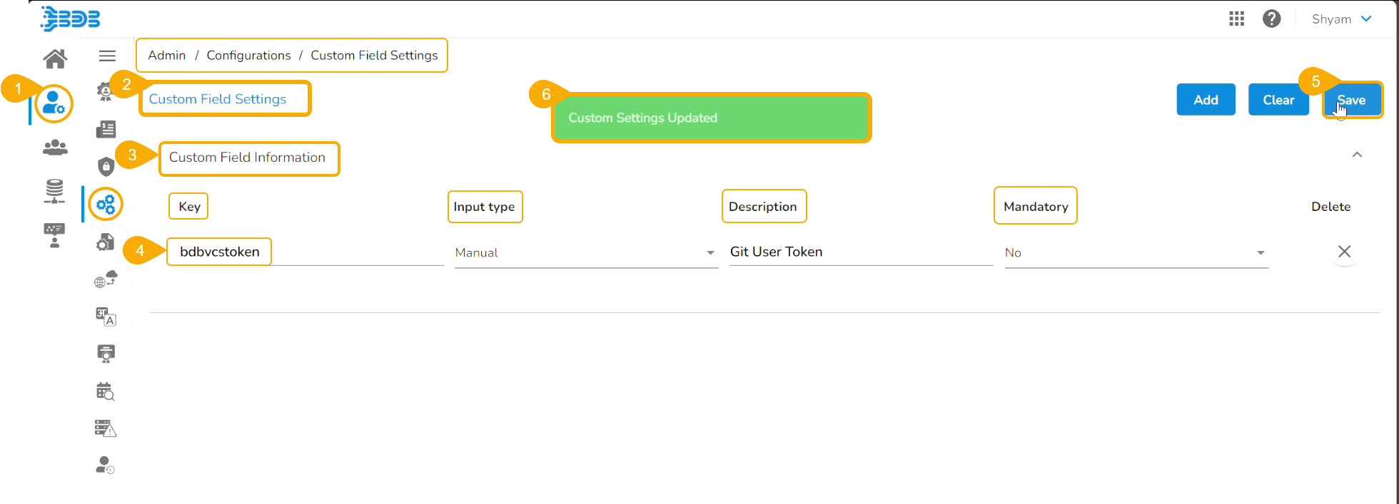
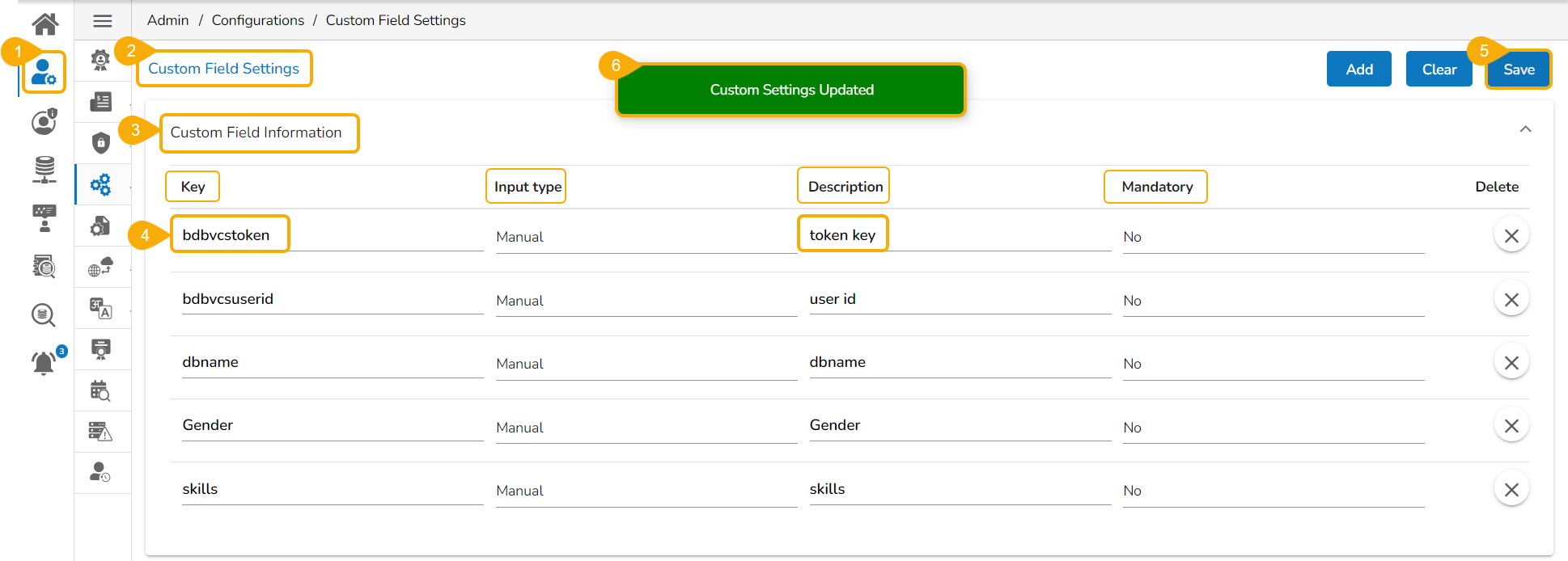
Configuring the Secret Management Administration option
Once the Secret Management has been configured from the Admin module it will have the Secret Key and related fields as explained in this section.
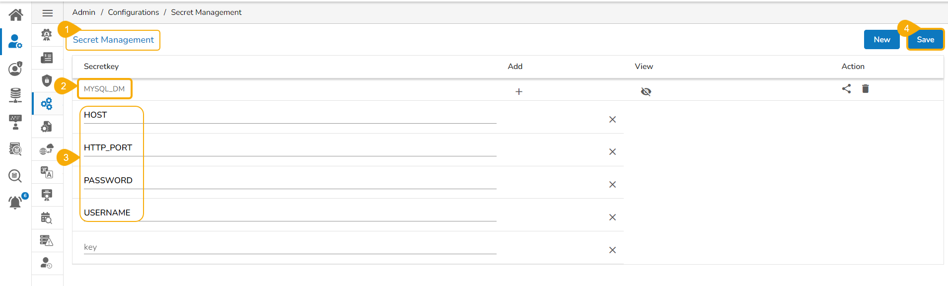
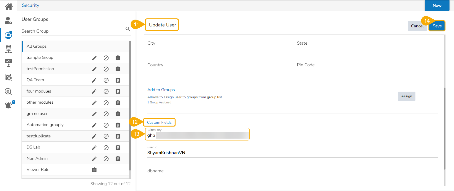
Navigate to the Secret Management option from the Admin module.
Add a Secret Key name.
Insert field values for the added Secret Key.
Please Note: The given image displays a sample Secret key name. The exact secret key name should be provided or configured by the administrator.
Share the configured Secret Management key to a user group.
Accessing the Secrets tab under a DS Notebook
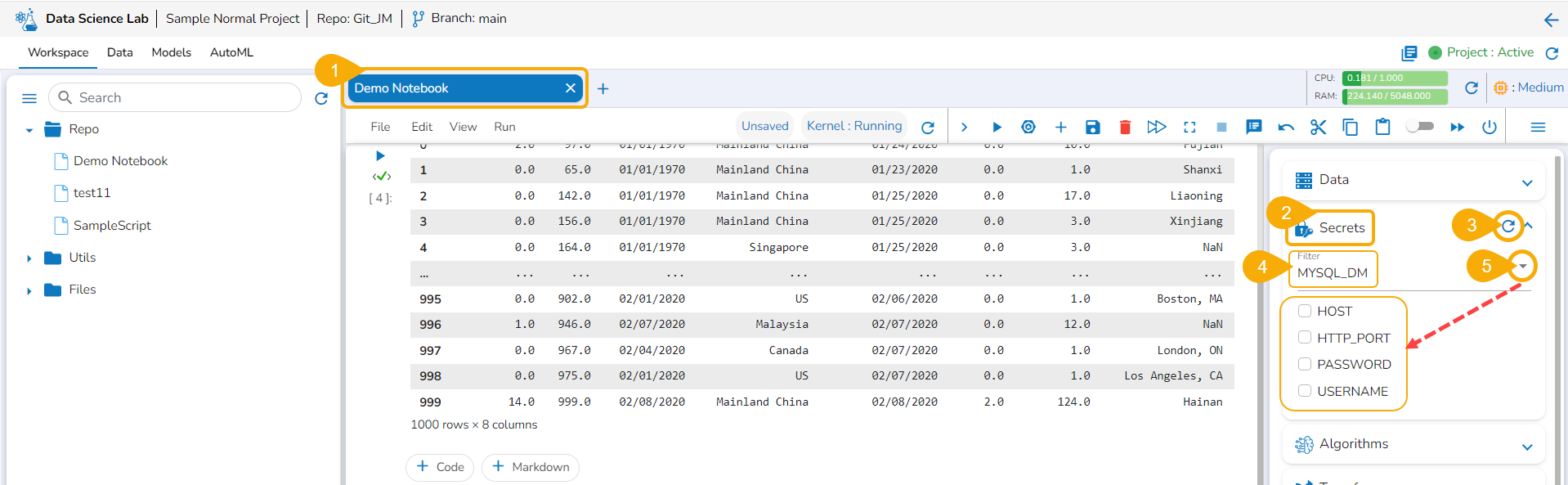
Access a Data Science Notebook from a user account that is part of the User group with which the configured secret is shared.
Open the Secrets tab from the right side.
Use the Refresh icon to get the latest configured Secret Key.
Add a new Code cell.
Select the Secret Keys by using the given checkboxes.
The encrypted environment variables for the fields are generated in the code cell.
Add a new Code cell.
Open the Writers tab.
Select a writer type using the checkbox. E.g., In this case, MySQL has been selected.
The data frame will be written to the selected writer's database.
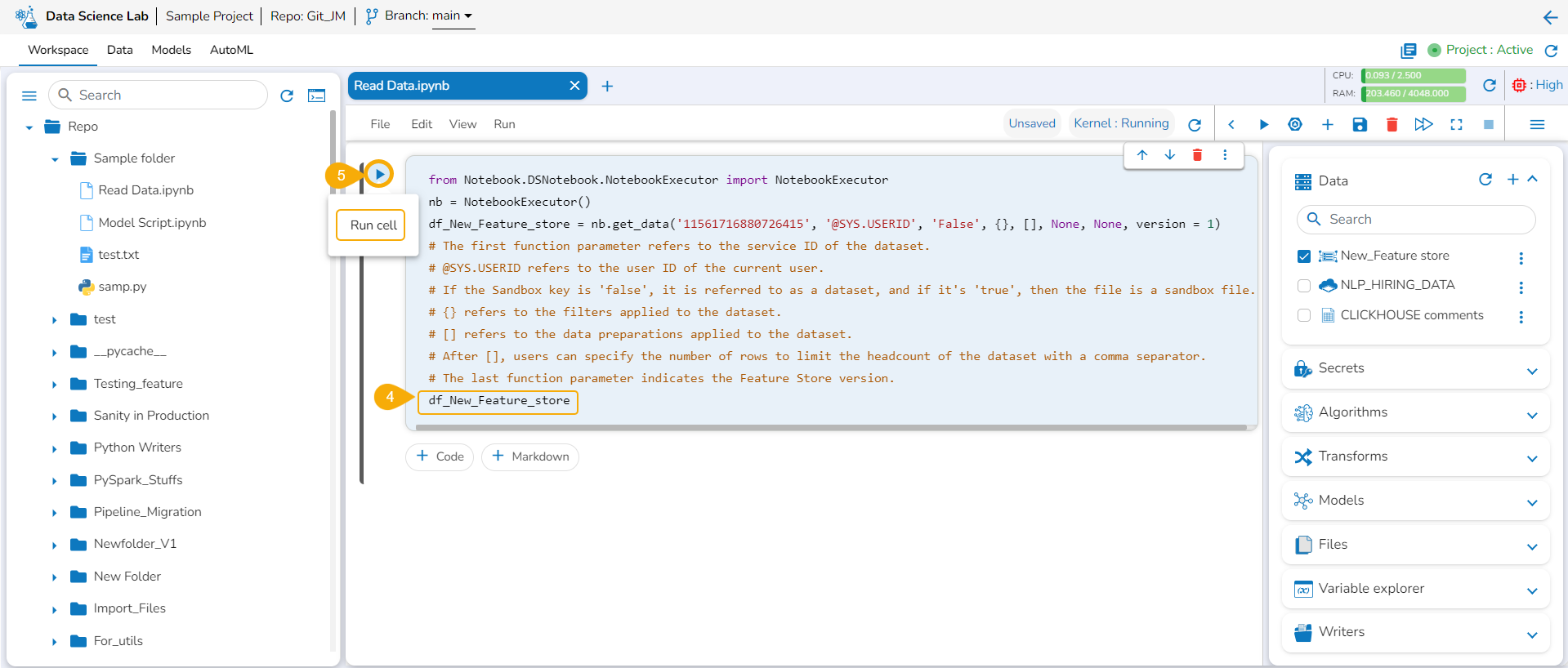
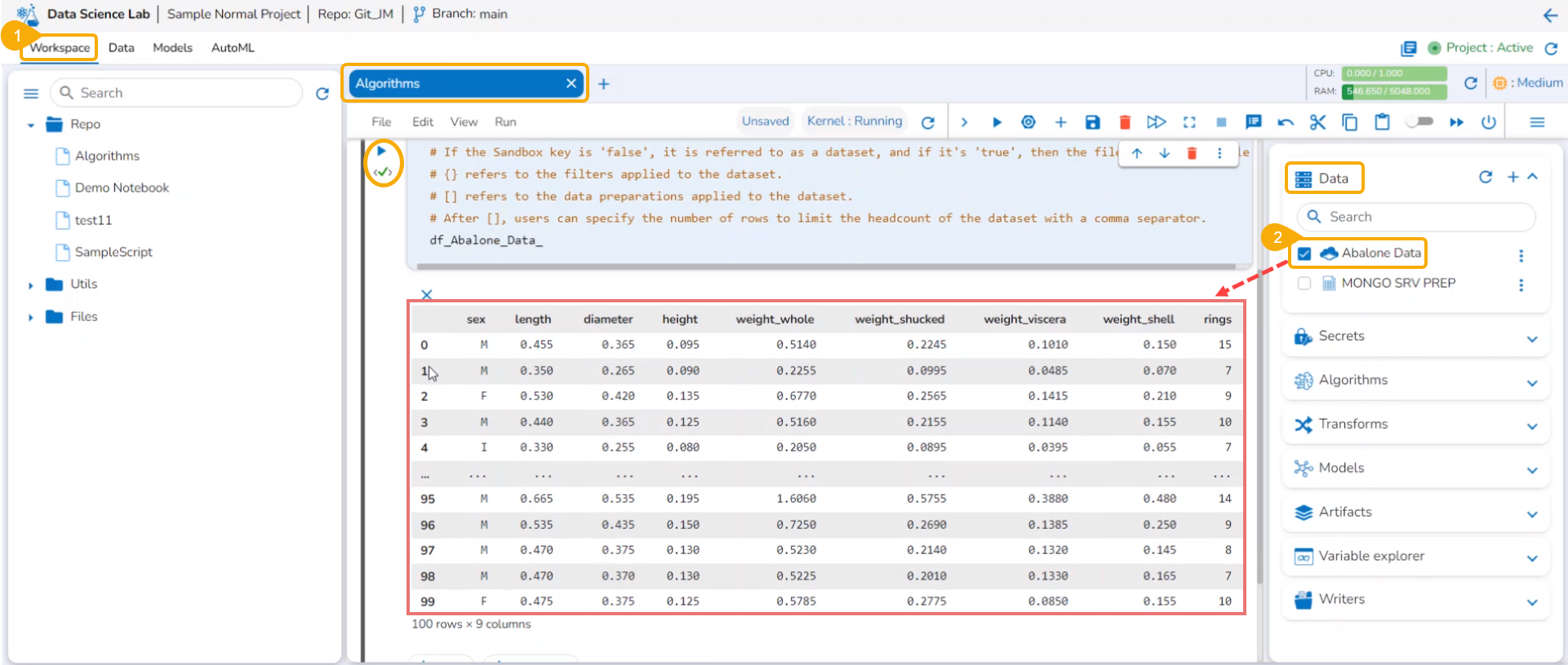
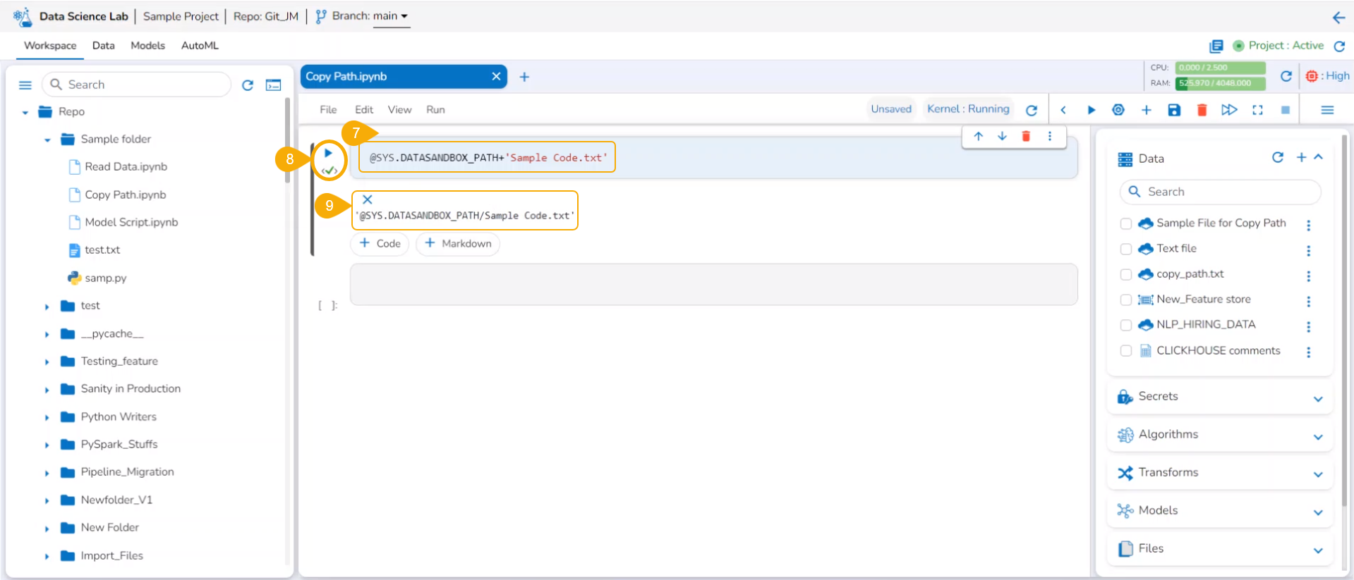
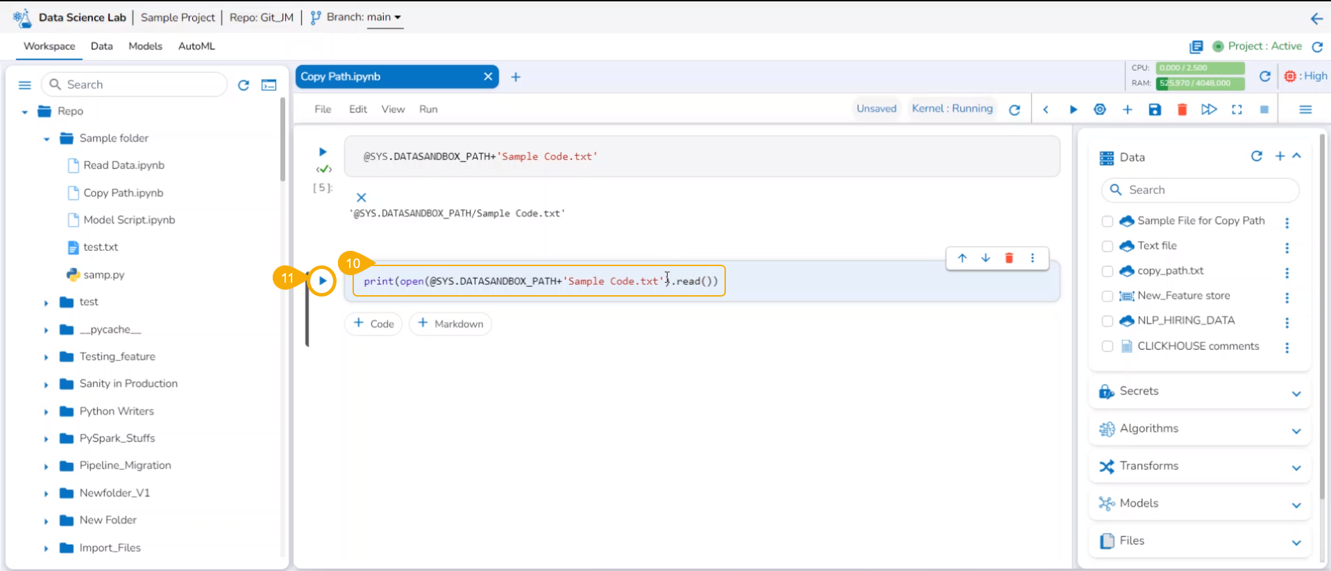
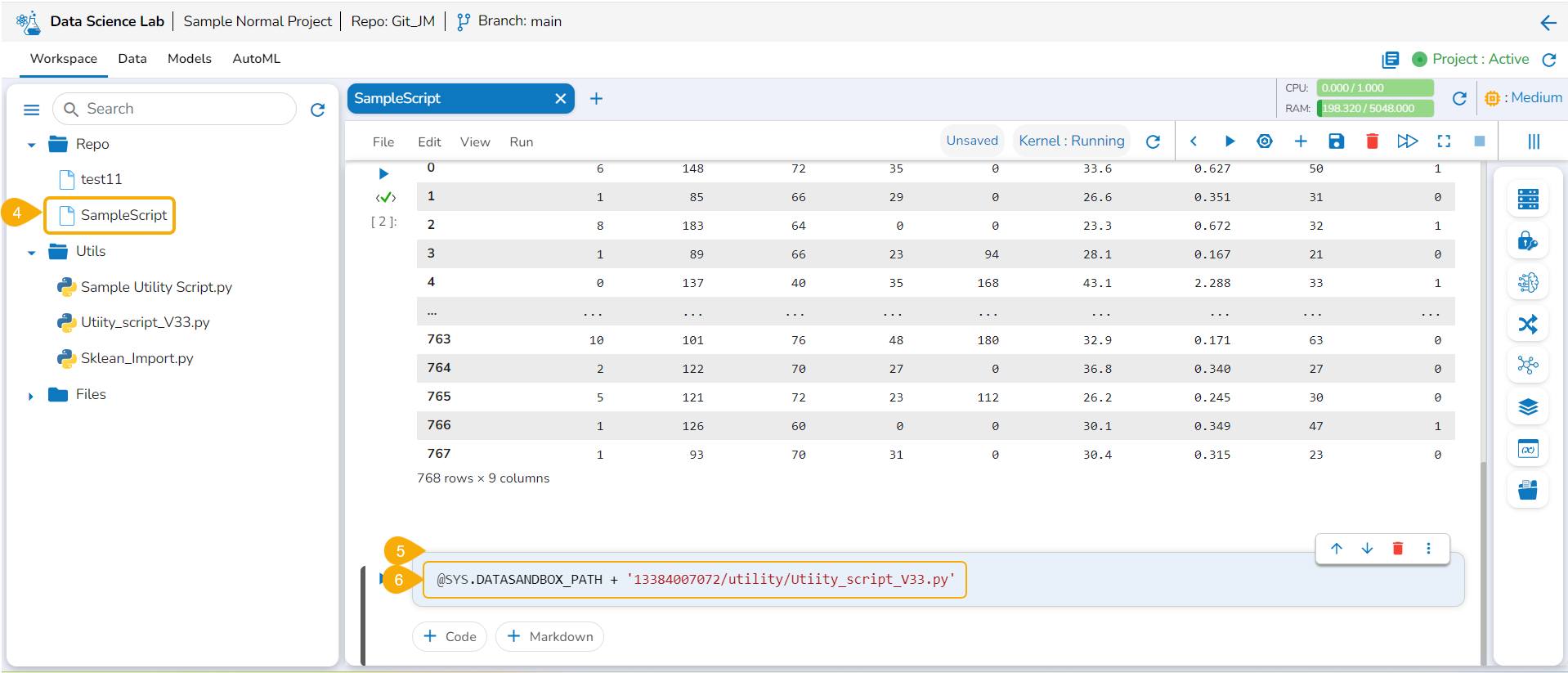
Reading Data
This section explains the steps to read the added Data inside a Data Science Notebook.
Reading the Added Data inside DSL Notebook
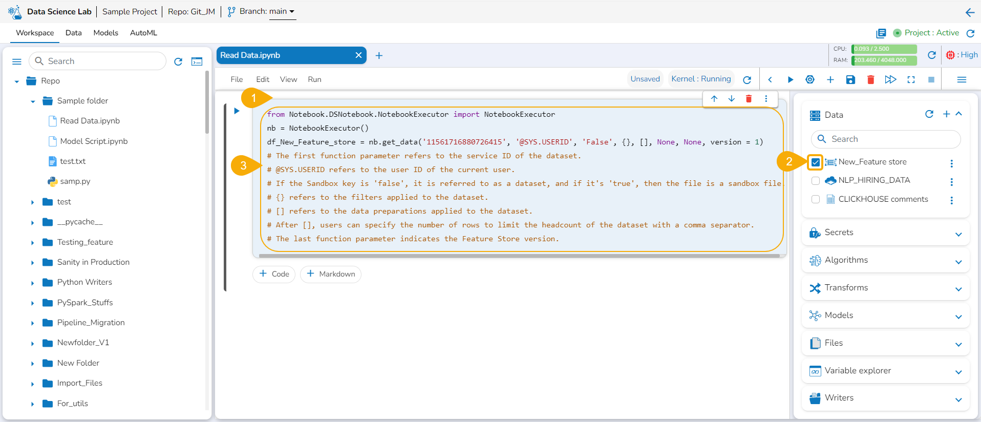
Please Note: Using the get_data function datasets and data sandbox files (csv & xlsx files) can be read.
Add a new Code cell to Notebook or access an empty Code cell.
Select a dataset from the Data tab.
The get_data function appears in the code cell.
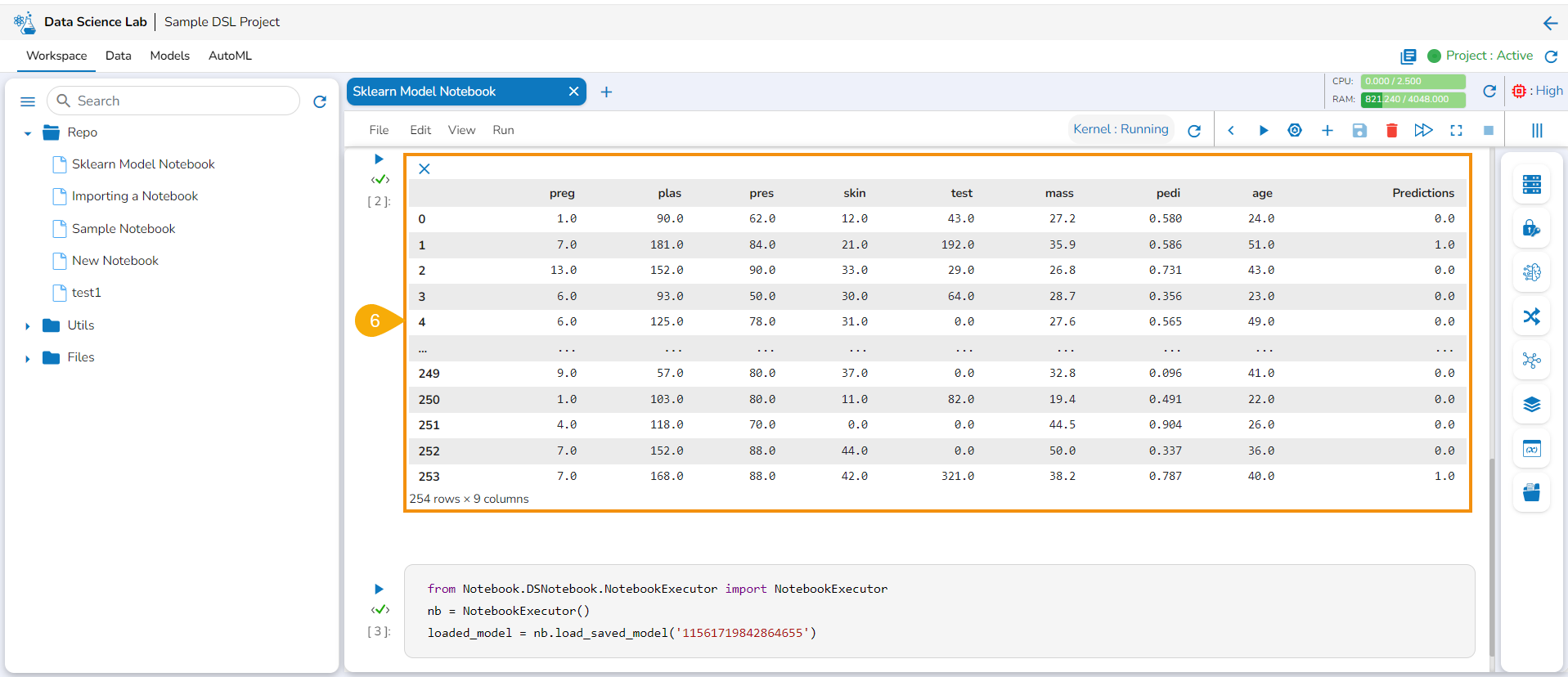
Provide the df (DataFrame) to print the data from the selected Dataset. A Dataset can be an added dataset, data sandbox file, or feature store.
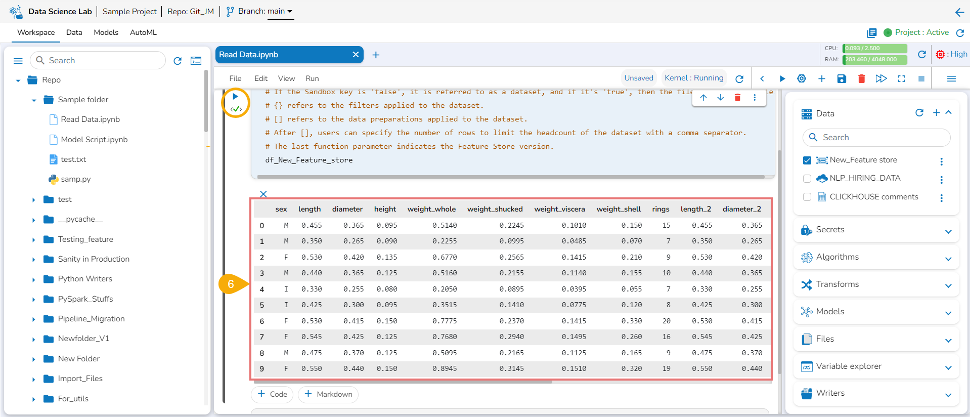
Run the cell.
The Data preview appears below after the cell run is completed.
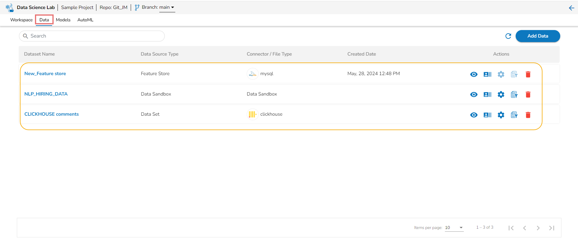
Project Level Data Tab
The Data Sets/ Sandbox files/ Feature Stores added to a Data Science Notebook will also be listed under the Data tab provided under the same project. Hence, the added datasets will be available for all the Data Science Notebooks created or imported under the same project.
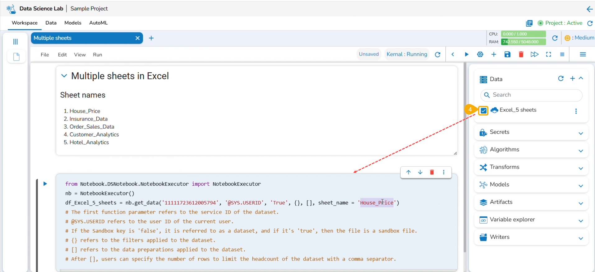
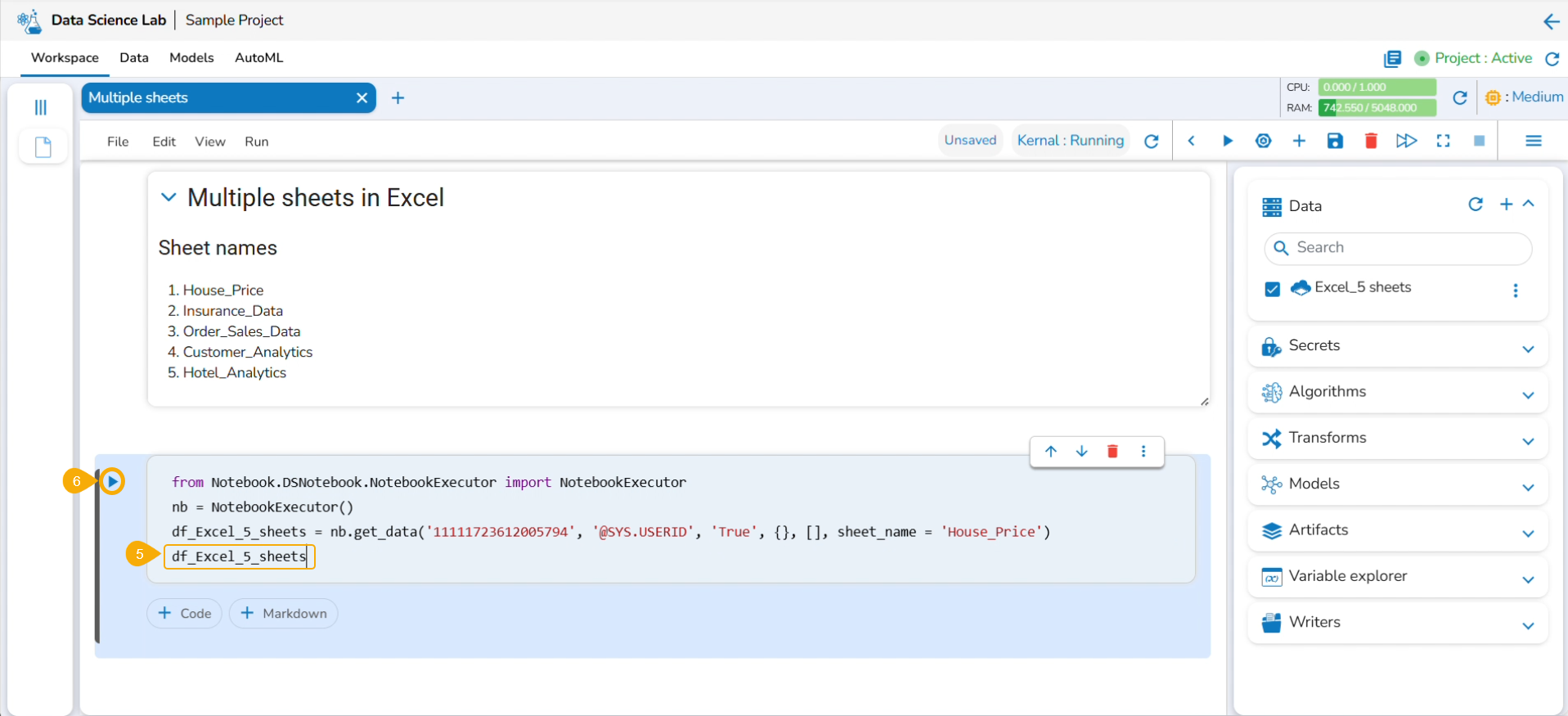
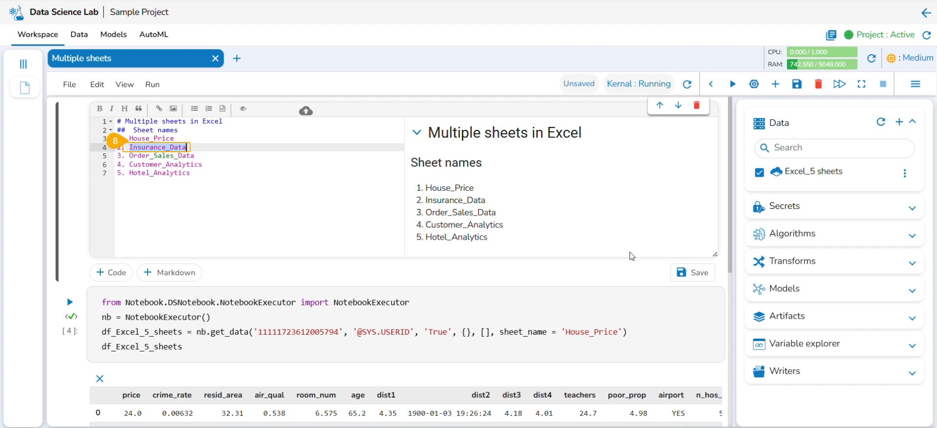
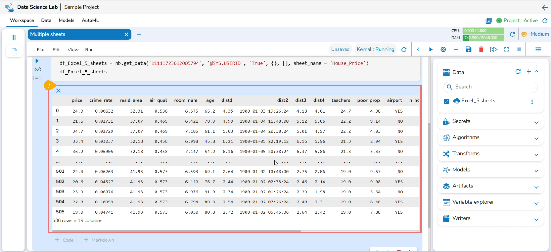
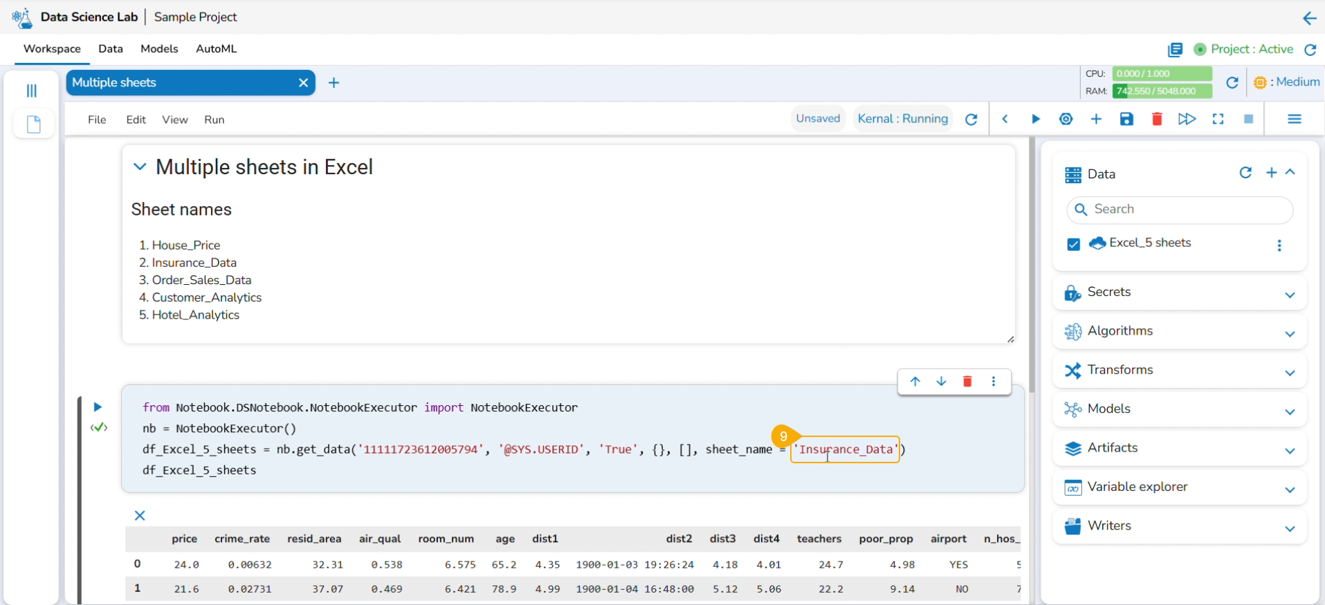
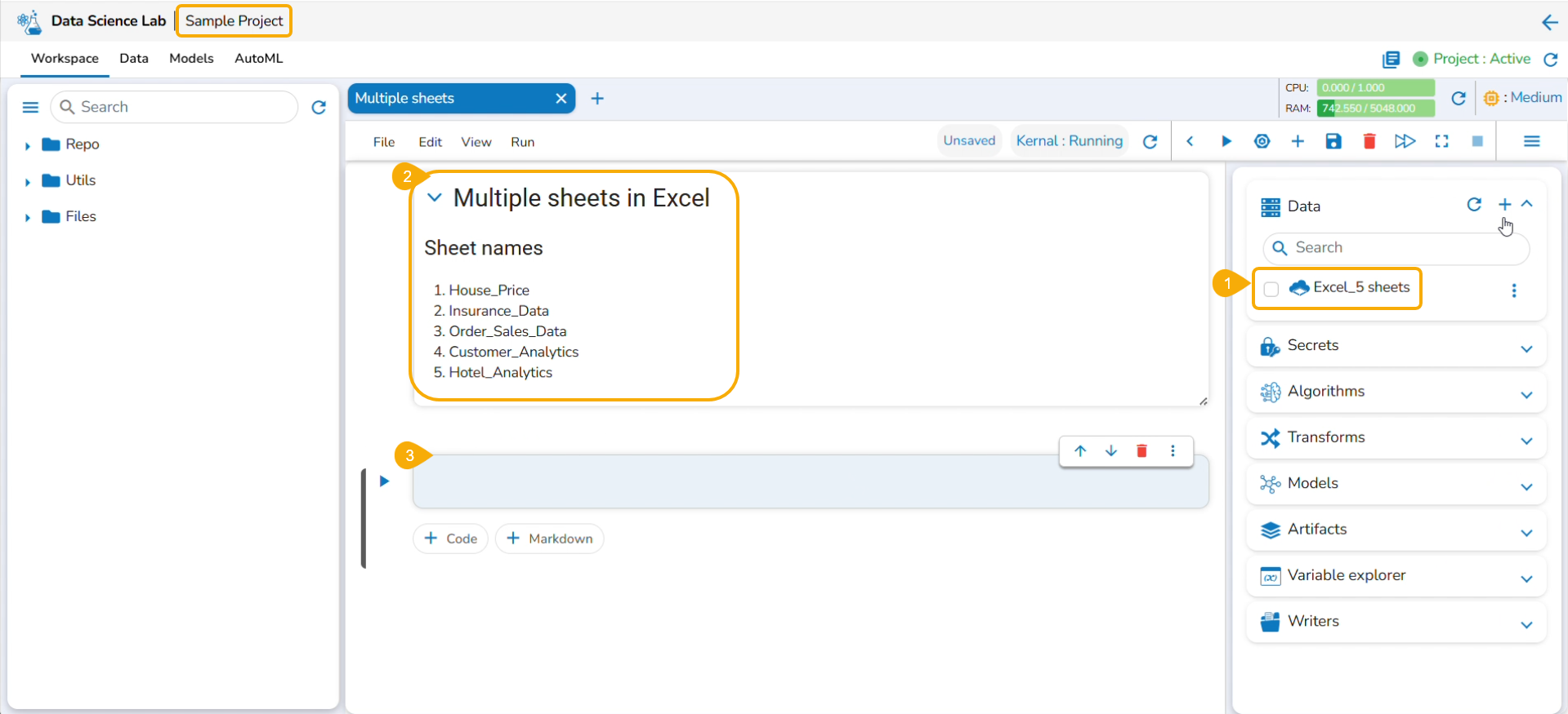
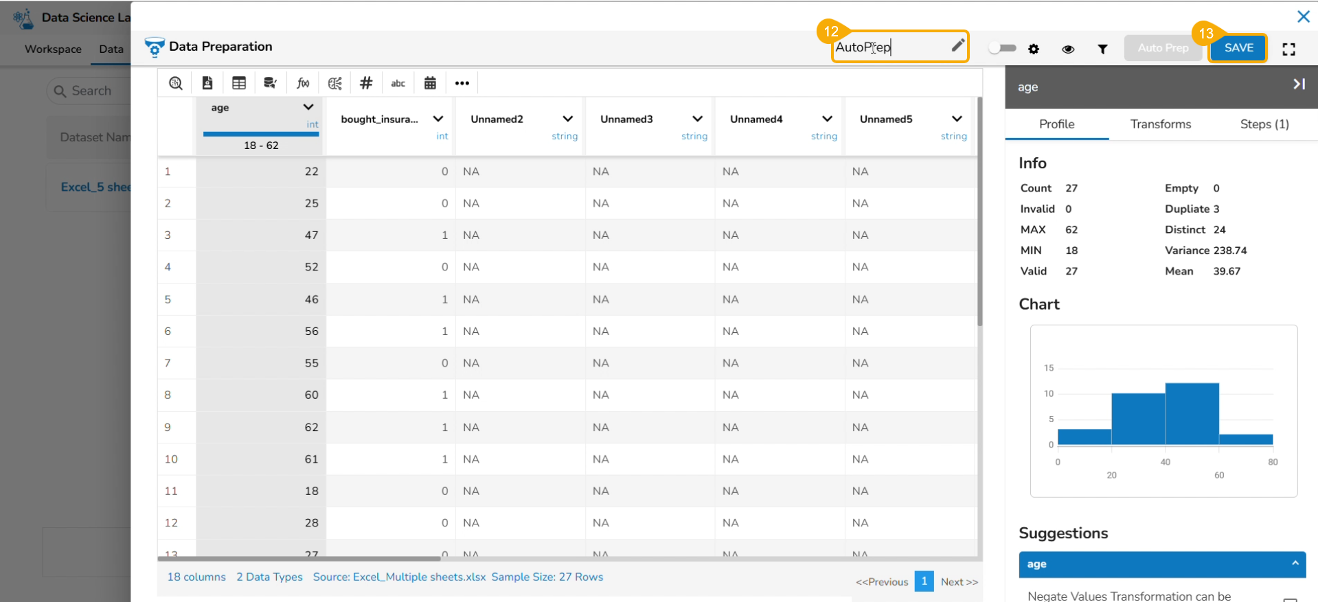
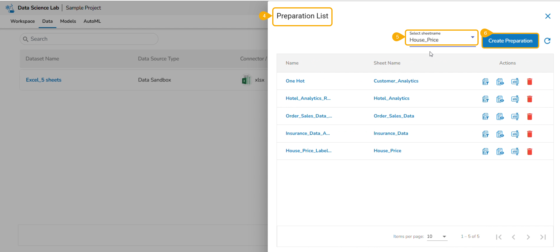
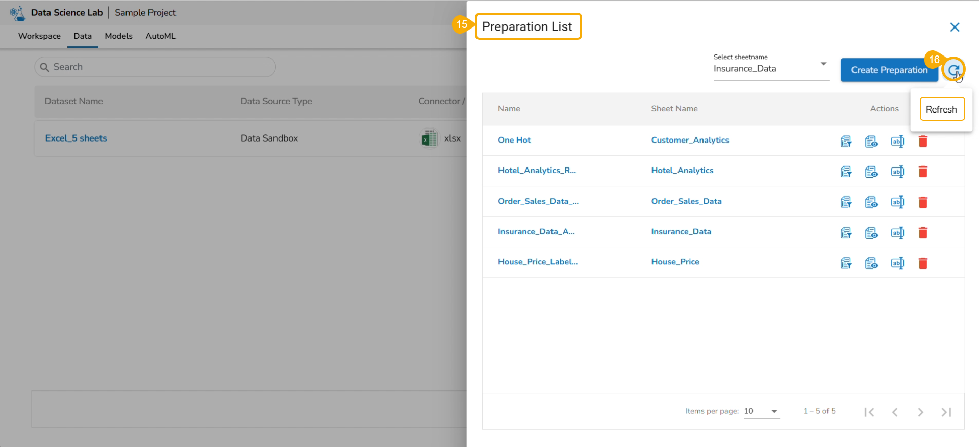
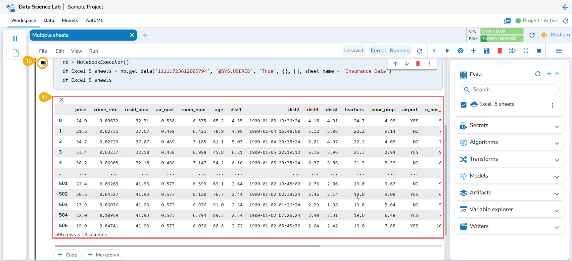
Reading Multiple Sheets inside an Excel Sheet
Check out the illustration to read multiple sheets in a Notebook cell.
Add an Excel file with multiple sheets to a DS Project.
Insert a Markdown cell with the names of the Excel sheets.
Insert a new code cell.
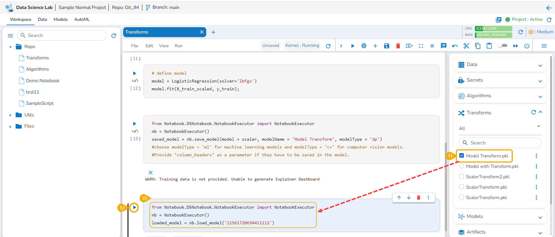
Transforms
Save and load models with transform script, register them or publish them as an API through DS Lab module.
Check out a walk-through on how to use the Transform script inside Notebook.
You can write or upload a script containing the transform function to a Notebook and save a model based on it. You can also register the model as an API service. This entire process is completed in the below-given steps:
Saving and loading a Model with Transform script
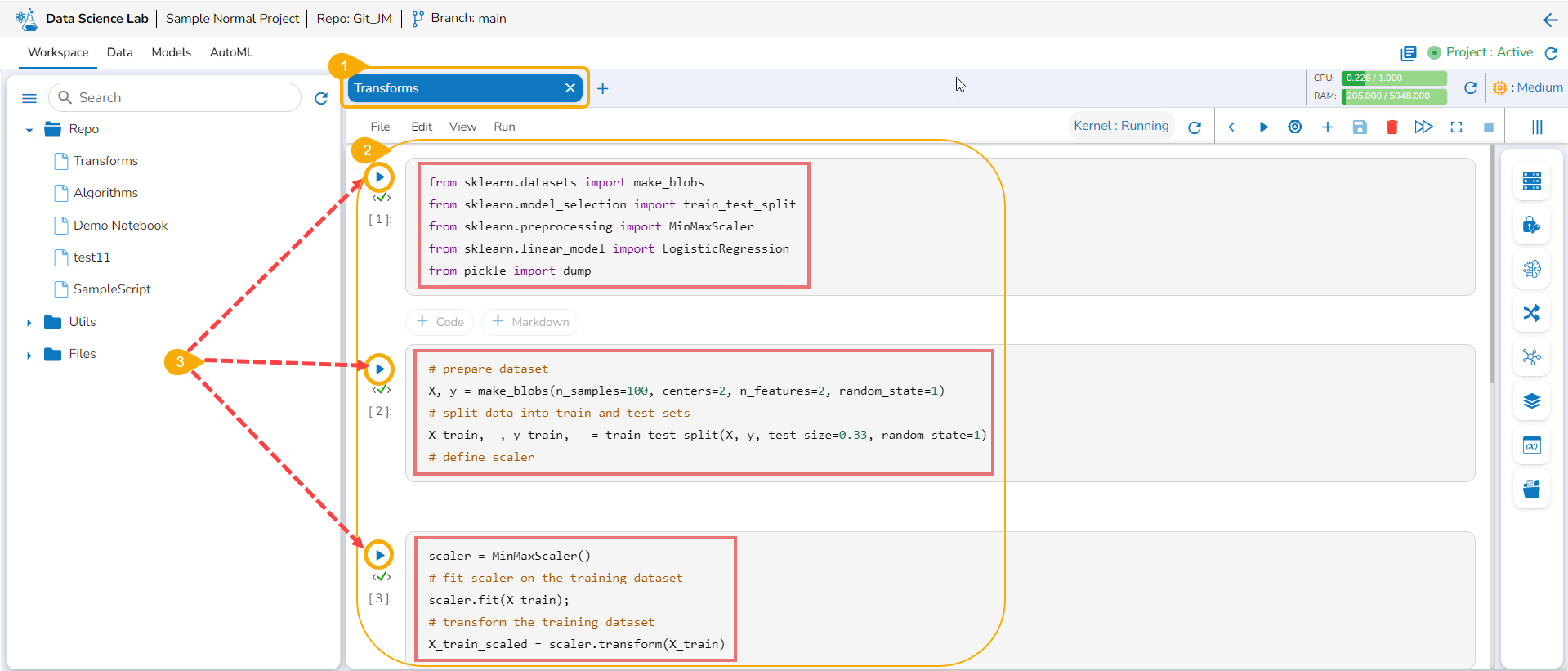
Navigate to a Notebook.
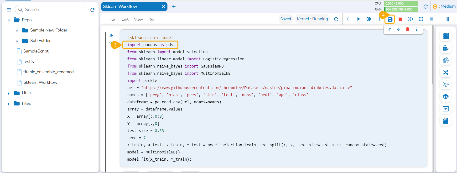
Add a Code cell. Write or provide a transform script to the cell (In this case, it has been supplied in three cells).
Run the cell(s) (In this case, run all the three cells).
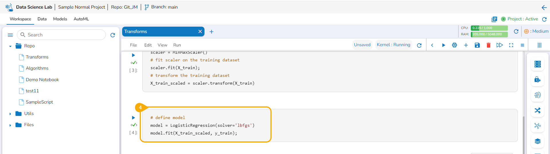
Add a new code cell and define the model.
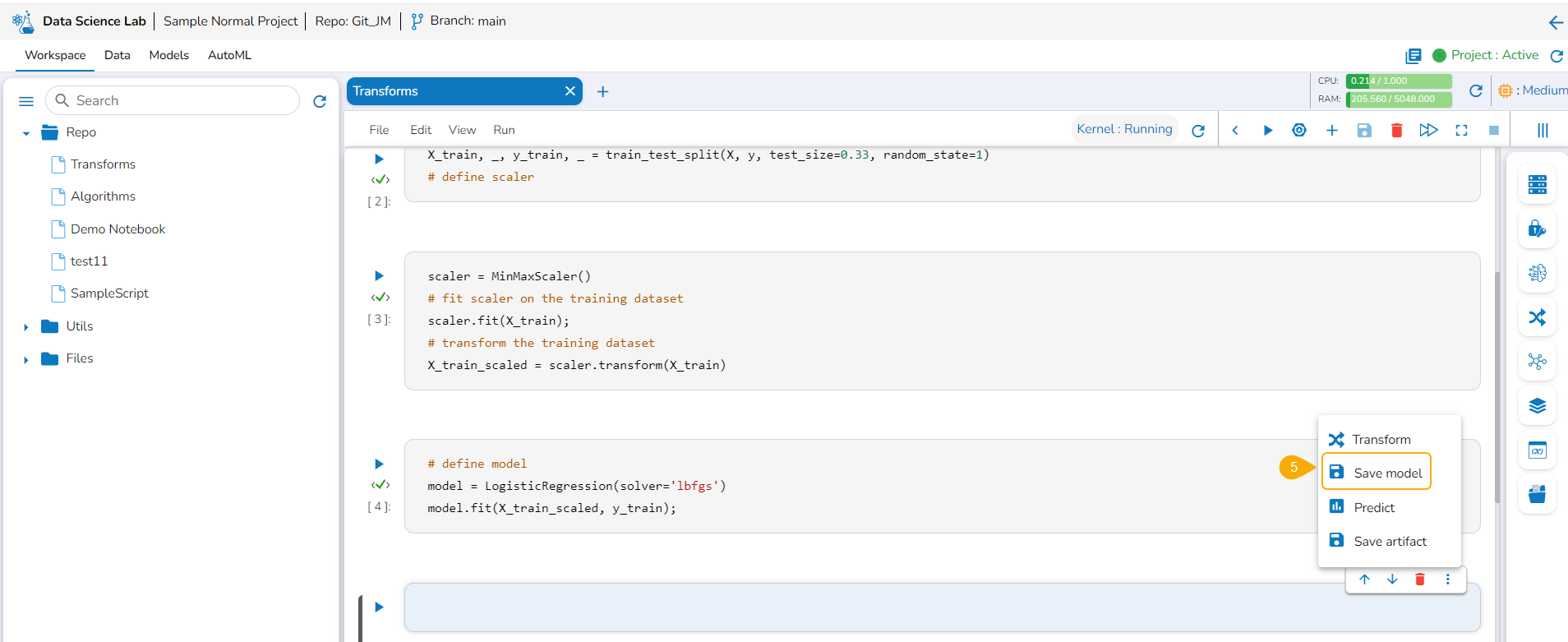
Add another cell and click the Save Model option for the newly added code cell.
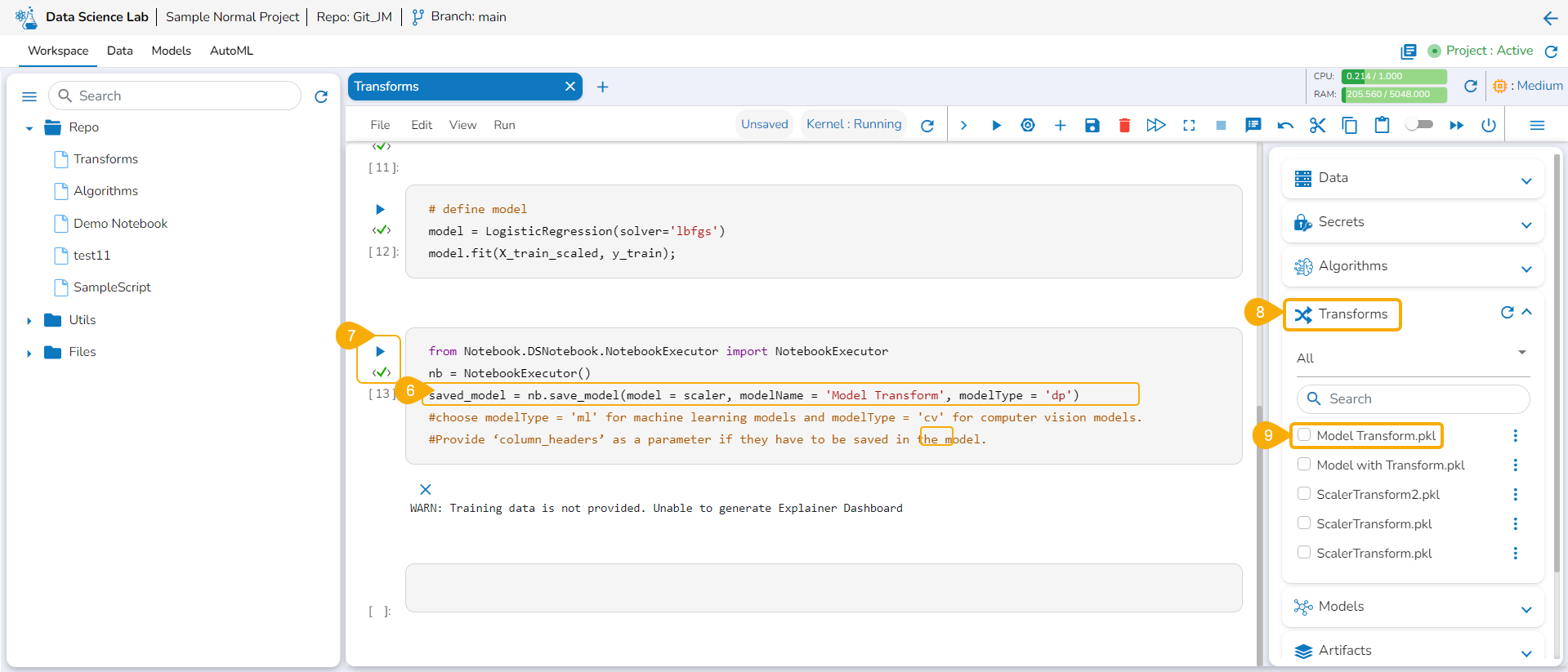
Specify the model name and type in the auto-generated script in the next code cell.
Run the cell.
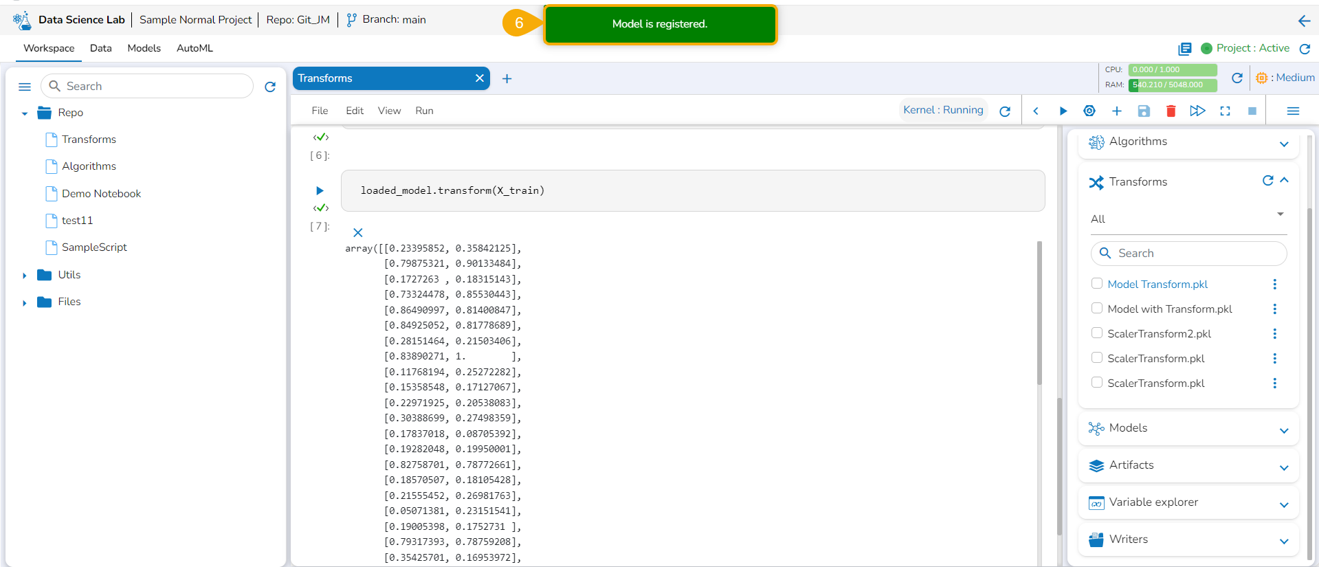
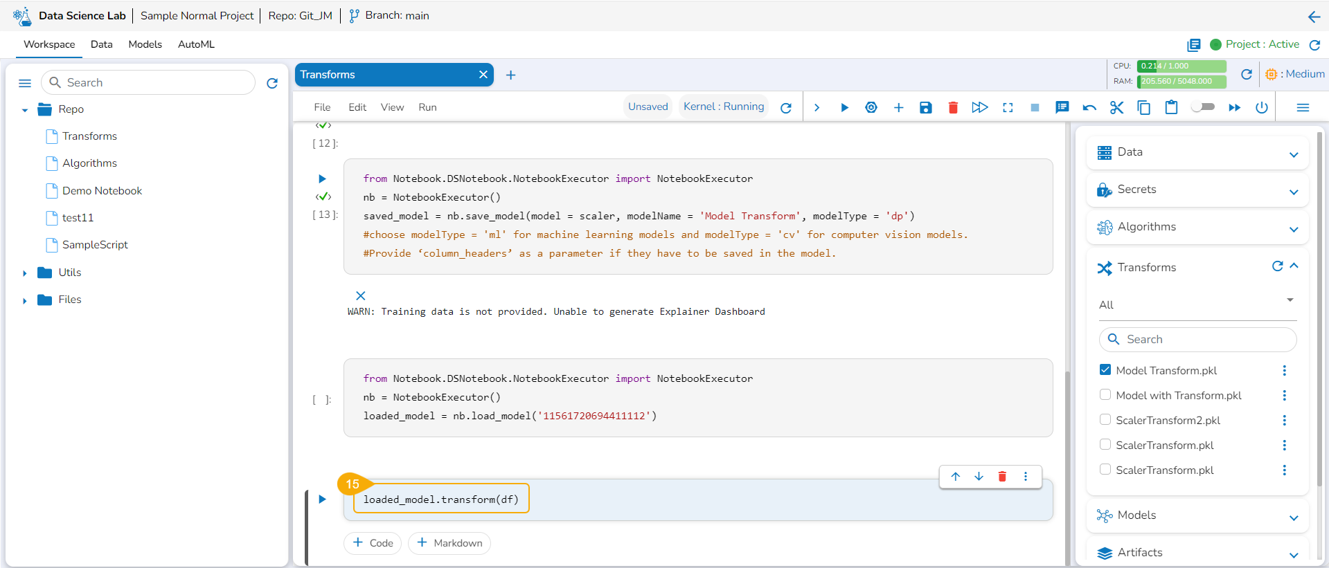
Open the Transforms tab.
Add a new code cell.
Load the transform model by using the checkbox.
Run that cell.
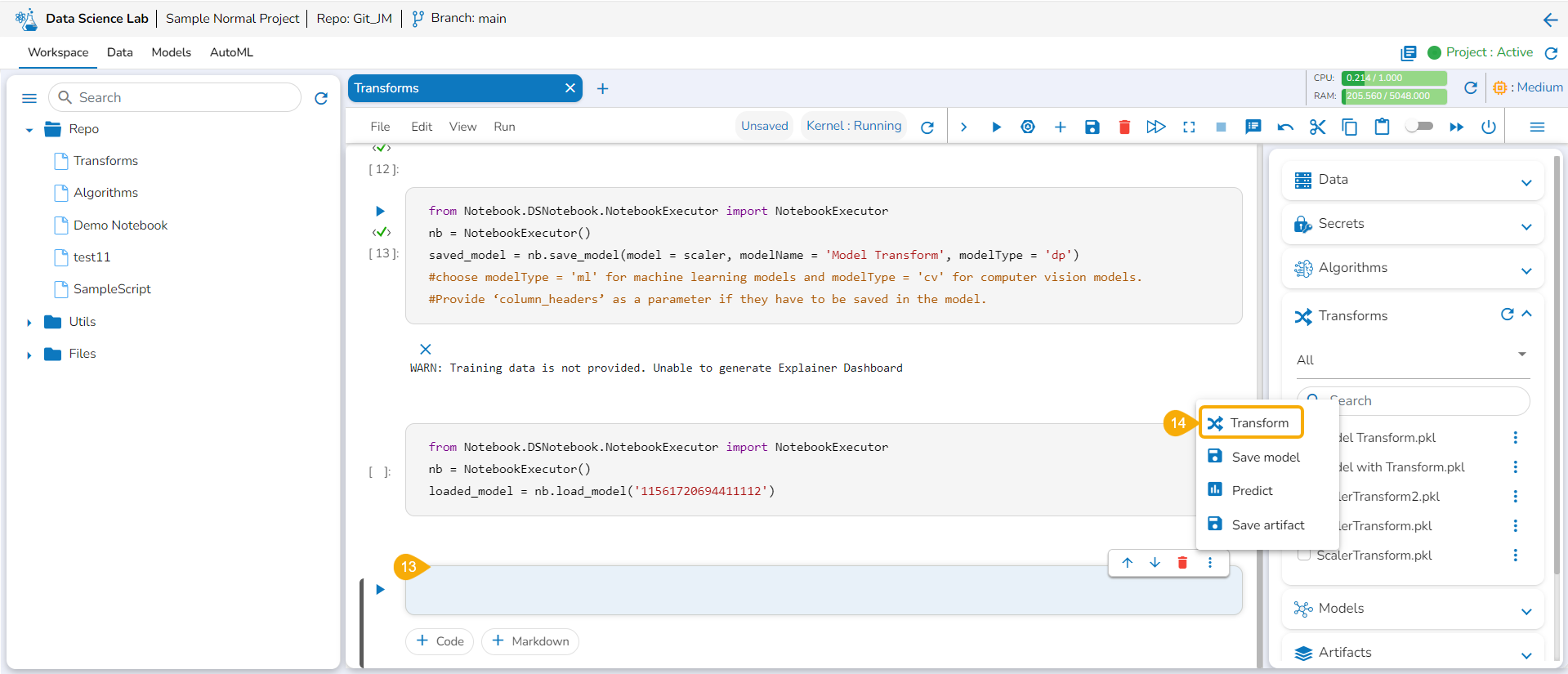
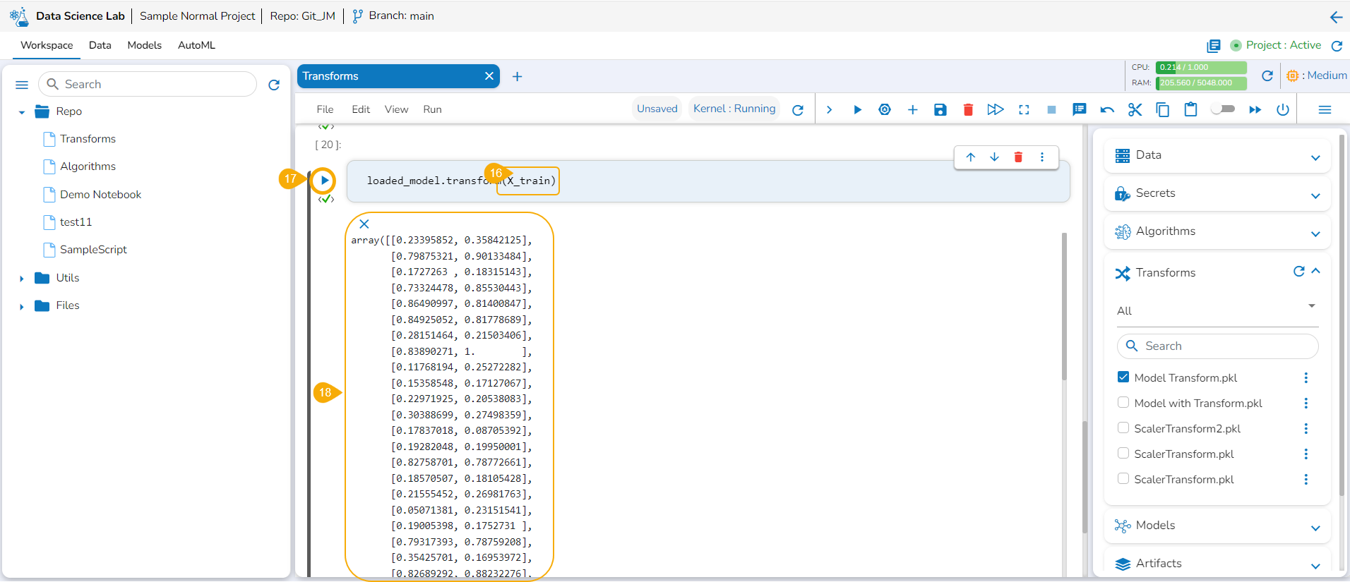
Insert a new code cell.
Click the Transforms option for the code cell.
The auto-generated script appears.
Specify the train data.
Run the code cell.
It will display the transformed data below.
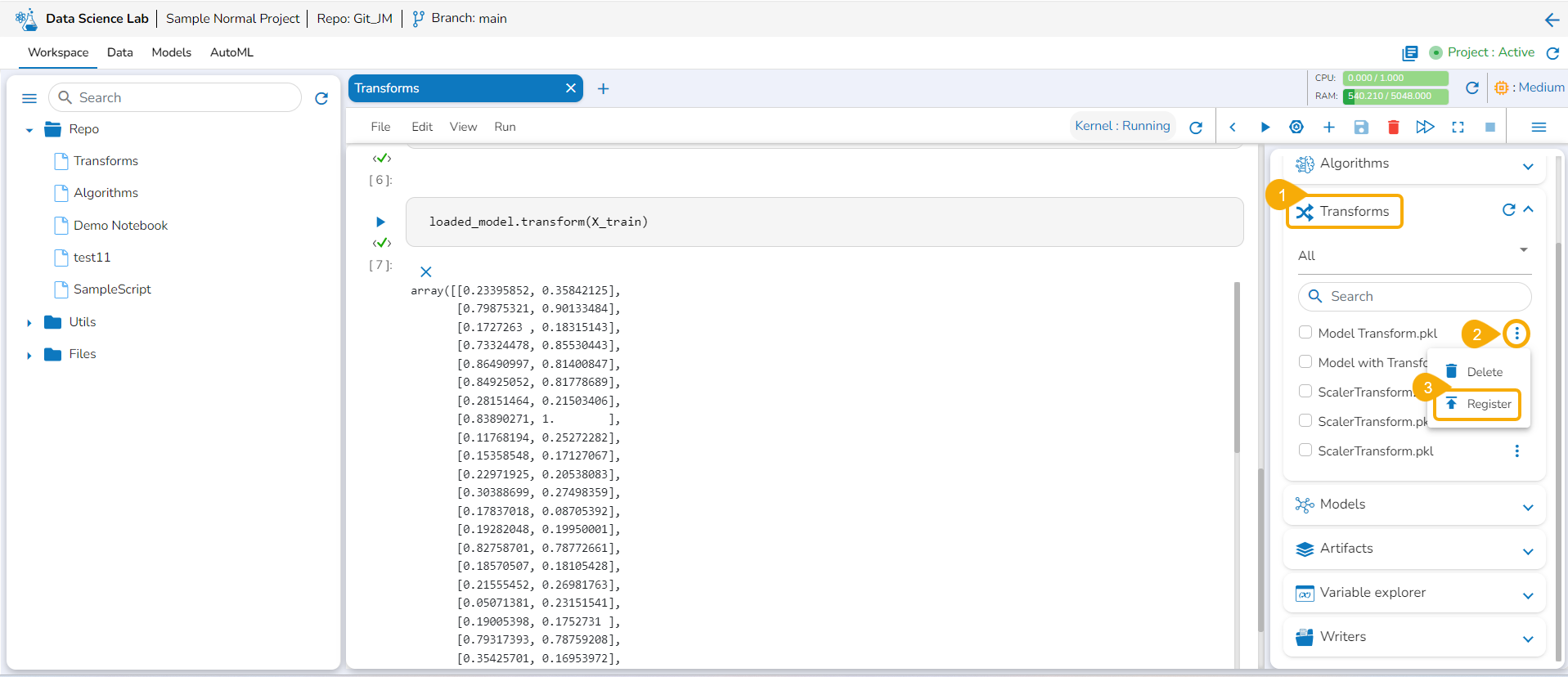
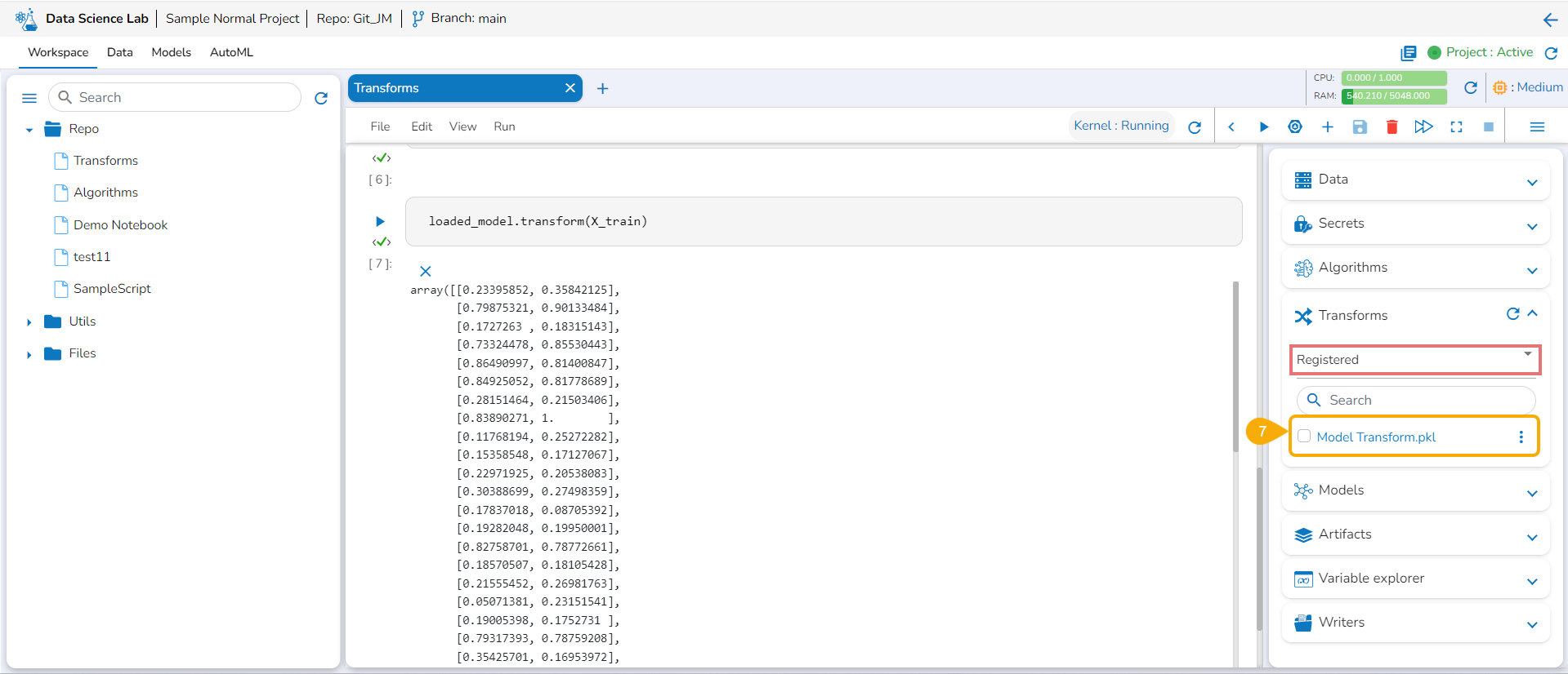
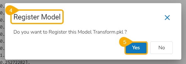
Registering a Transform Model
Open the Transforms tab inside a Notebook.
Click the ellipsis icon for the saved transform.
Select the Register option for a listed transform.
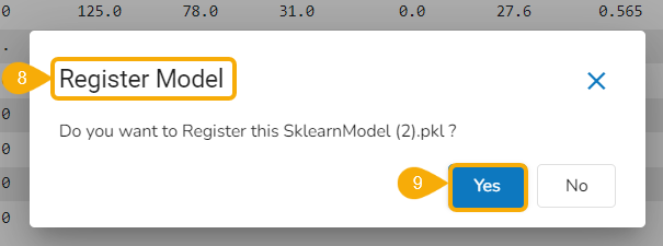
The Register Model dialog box opens to confirm the action.
Click the Yes option.
A confirmation message appears to inform the completion of the action.
The model gets registered and listed under the Registered list of the models.
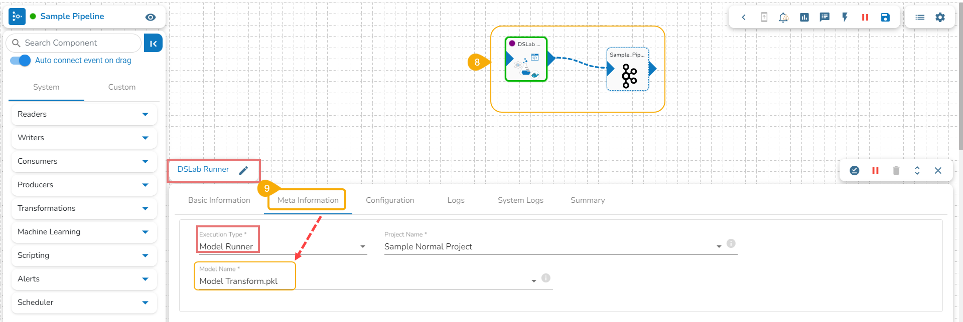
Open a pipeline workflow with a DS Lab model runner component.
The registered model gets listed under the Meta Information tab of the DS Lab model runner component inside the Data Pipeline module.
Publishing a Transform Model as API
The steps to publish a model as an API that contains transform remain the same as described for a Data Science Model. Refer to the
Create Feature Store
What is a Feature Store?
A Feature Store is a centralized repository for storing, managing, and sharing machine learning (ML) features or attributes used to train models. It is a scalable solution for organizing and cataloging features, making them easily accessible to data scientists and ML engineers across an organization. Feature Stores facilitate collaboration, version control, and reusability of features, streamlining the ML development process and improving model quality and efficiency.
Using a Code Cell
Write & Run Code to create Data Science Scripts and models using the .ipynb file.
A user can write and execute code using the Data Science Notebook interface. This section covers the steps to write and run a sample code in the Code cell of the Data Science Notebook.
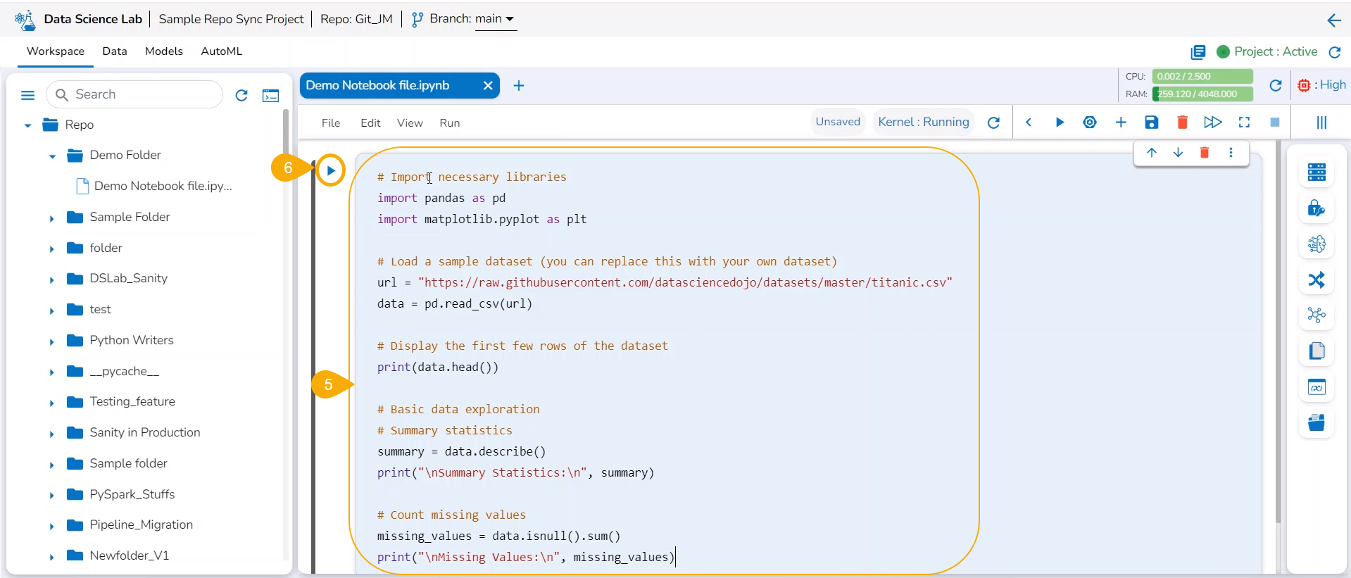
Check out the given walk-through on how to use a Code Cell under a .ipynb file.
Regression Model Explainer
This page provides model explainer dashboards for Regression Models.
Check out the given walk-through to understand the Model Explainer dashboard for the Regression models.
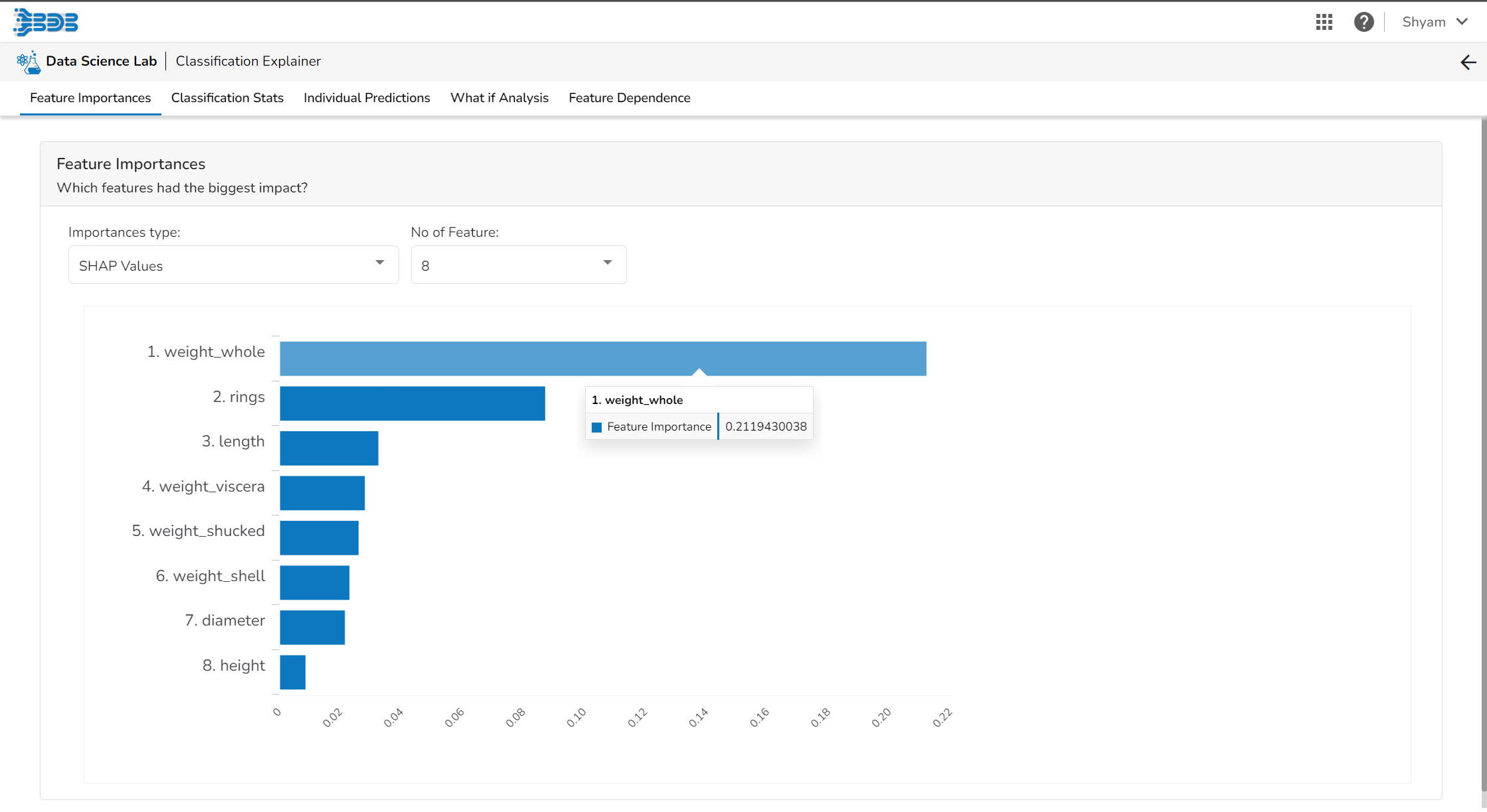
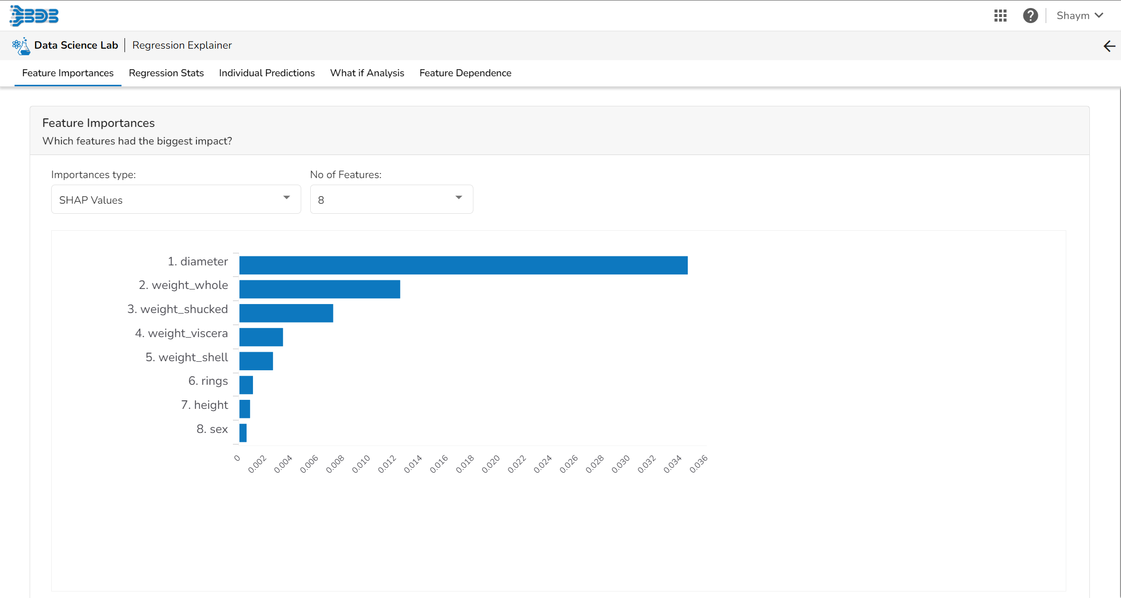
Feature Importance
Provide Description (optional).
Select a Target Column.
Select a Data Preparation from the drop-down menu.
Use the checkbox to select a Data Preparation from the displayed drop-down.
Select columns that need to be excluded from the experiment.
Use the checkbox to select a field to be excluded from the experiment.
Please Note: The selected fields will not be considered while training the Auto ML model experiment.
Click the Next option.
Click the Done option.
AutoML experiment with Started Status
Experiment with Started Status
Experiment with Running Status
Experiment with Completed Status
Description
Click the Save option.
The newly created Notebook is ready now for the user to commence Data Science experiments. The newly created Notebook is listed on the left side of the Notebook page.
The accessible datasets, models, and artifacts will be listed under the
Datasets
,
Models
, and
Artifacts
menus.
The Find/Replace menu facilitates the user to find and replace a specific text in the notebook code.
The created Notebook (.ipynb file) gets added to the Repo folder. The Notebook Actions are provided to each created and saved Notebook. Refer to the Notebook Actions page to get detailed information.
Create Option for a new Notebook Creation
Add icon provided for a Notebook
Create Notebook Drawer
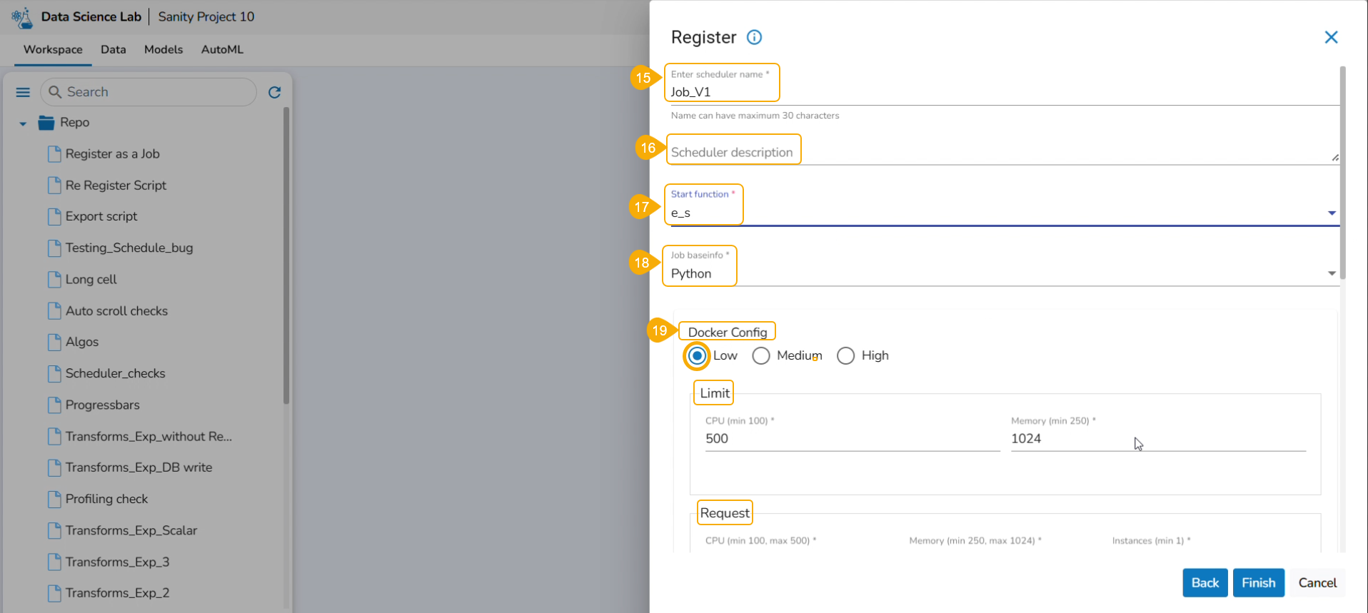
Execution Type: Select the Script Runner option.
Function Input Type: Select one option from the given options: Data Frame or List.
Project Name: Select the Project name using the drop-down menu.
Script Name: Select the script name using the drop-down menu.
External Library:Mention the external library.
Start Function: Select a function name using the drop-down menu.
The exported Script is displayed under the Script section.
Accessing an Exported Script inside the DS Lab Script Runner Component
Click the Save option to save the Secret Management configuration.
The newly created Secret Keyis listed below. Click on a Secret Key option.
The selected Secret Key name option is displayed with a drop-down icon. Click the drop-down icon next to the Secret Key name to get the fields.
Map the encrypted secret keys for the related configuration details like Username, Password, Port, Host, and Database by copying them.
Check out the illustration to create a new Feature Store.
Steps to Create A Feature Store
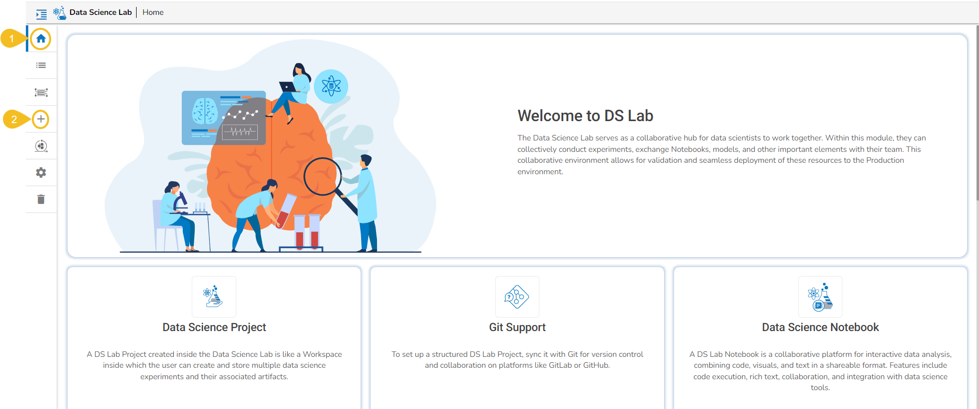
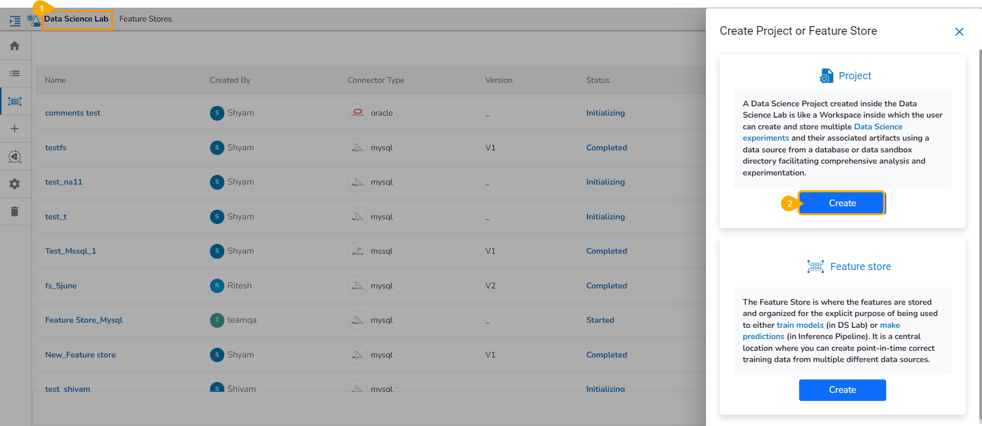
Navigate to the Homepage of the Data Science Lab module.
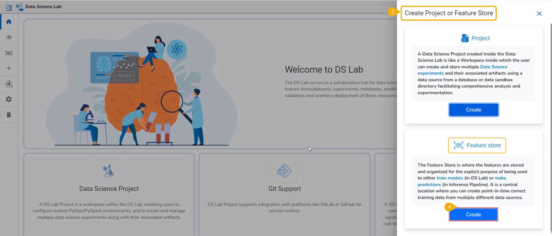
Click the Create icon from the homepage.
Accessing the Create icon
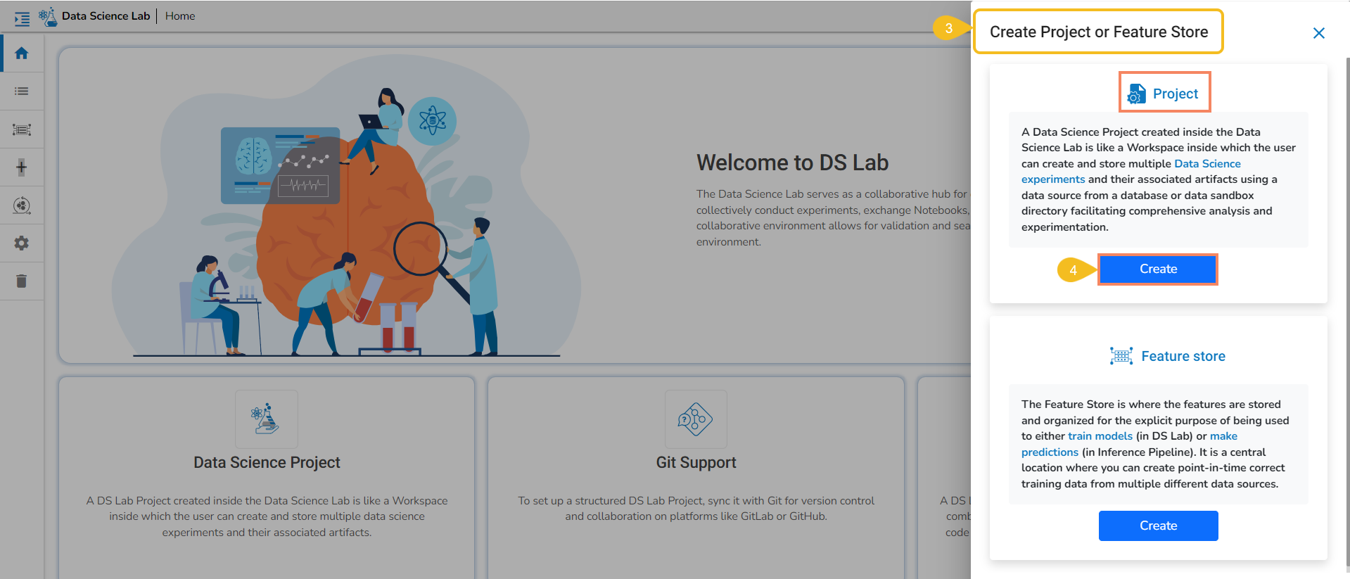
The Create Project or Feature Store drawer opens.
Click the Create option provided for the Feature Store.
Create Project/ Feature Store window
The Create Feature Store page opens.
Provide a name for the Feature Store.
Select a Data Connector from the drop-down list.
The Table info/ metadata panel will appear on the right side of the page.
Click on a table name to select it.
An SQL query will be generated in the given place.
Click the Validate option.
A notification message ensures the user that the action has been executed successfully and the table is executed.
A preview of the table appears below.
Click the Create option.
A notification message ensures the user that the intended Feature Store is being created.
The user gets redirected to the Feature Stores page.
The newly created Feature Store gets added at the top of the list.
Feature Stores List with newly created Feature Store
Please Note:
Click the Refresh icon to get the status level updates for the newly created Feature Store.
A Feature Store gets Initializing, Started, and Completed as Status.
Scheduling a Feature Store
Check out the illustration on scheduling a Feature Store.
Navigate to the Data Science Lab module.
Click the Create option provided for Feature Store.
The Create Feature Store form opens.
Provide the Featureset Name.
Select a connector using the drop-down menu.
Write or get an SQL query by selecting a table/metadata from the Tab Info./Metadata panel.
Validate the query using the Validate option.
A notification appears to ensure the user after the query is validated.
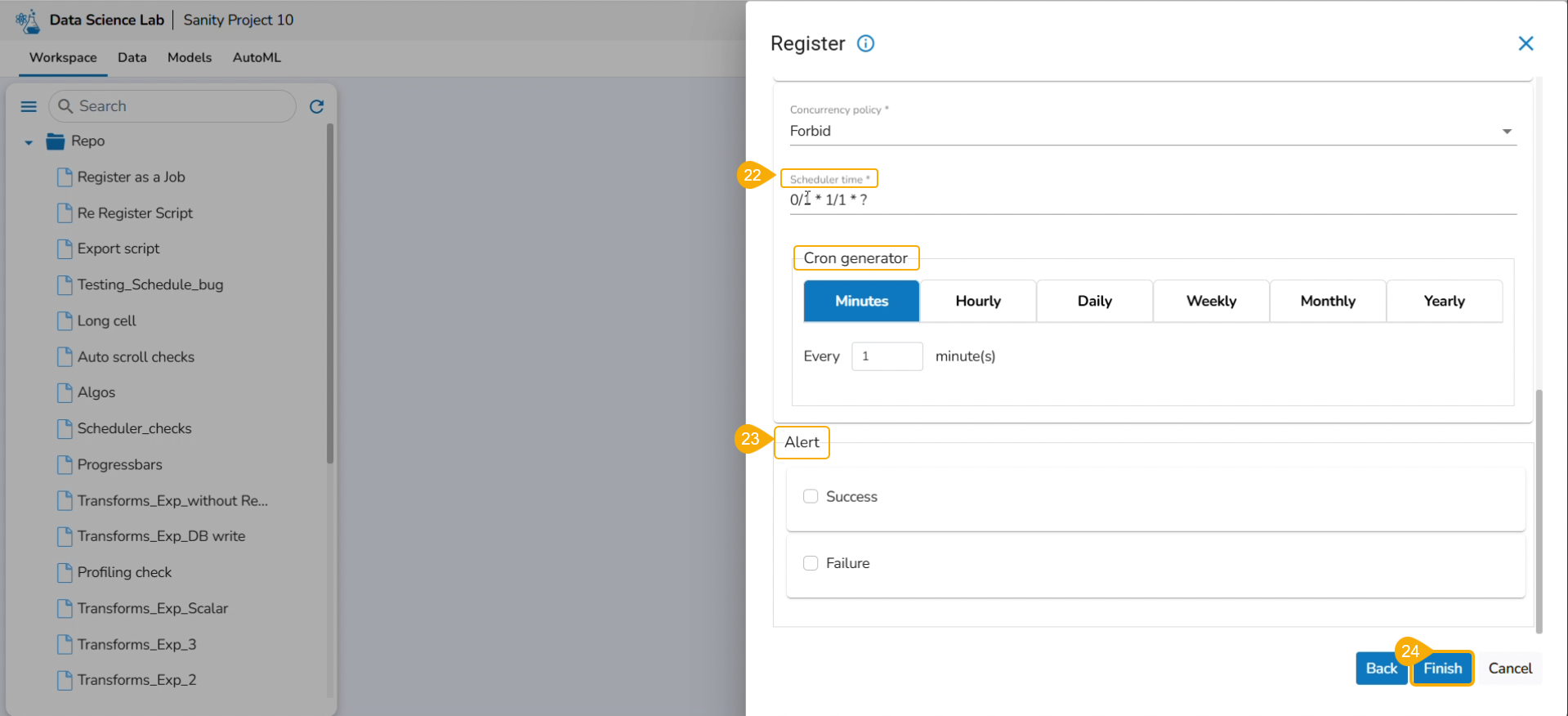
Click the Schedule option.
The Schedule page appears.
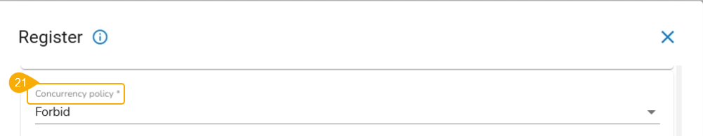
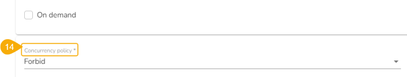
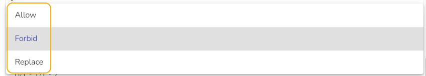
Select an option for theConcurrency Policy. The following options are provided:
Allow (Parallel): Multiple instances run simultaneously. No concurrency restrictions. Suitable for independent tasks.
Forbid (Prevent, Deny): Only one instance runs simultaneously. New instances are skipped if a previous one is running. Suitable for tasks that can't run in parallel.
Replace (Terminate, ReplaceOlder): A new instance starts, previous one is terminated. Suitable when the latest instance should take priority. Ensures no overlap.
Navigate to the Cron Generator section.
Choose the Monthly or Yearly option and provide the required information.
Based on the selection from the Cron Generator the Scheduler Time will be added.
Click the Apply option.
The user gets redirected to the Create Feature Store page, a notification ensures that the Feature Store is scheduled.
The same will be indicated through a green mark in the Scheduler option.
Click the Create option.
The user gets redirected to the Feature Stores page.
The newly created Feature Store is added at the top of the page.
A notification message ensures that the Feature store job is initialized. The same is suggested through the Status column.
Click the Refresh icon.
The feature store status gets changed to Started.
Click the Refresh icon.
The Feature Store status gets changed to Completed.
The Stop Scheduling icon gets enabled for the feature store.
Please Note: The Stop Schedule option will remain enabled when a scheduled Feature Store reaches the scheduled time limit. The user can click the Stop Schedule icon during this period to stop the schedule.
Please Note: The above-given video displays inserting a new code cell using the Add Pre-cell icon for a code cell.
Running Code inside a Code Cell
Create a new .ipynb file.
A notification message appears to ensure the creation of the new .ipynb file.
Open the newly created .ipynb file.
Insert the first Code cell by using the Add pre-cell icon.
Write code inside the cell.
Click the Run cell icon to run the code.
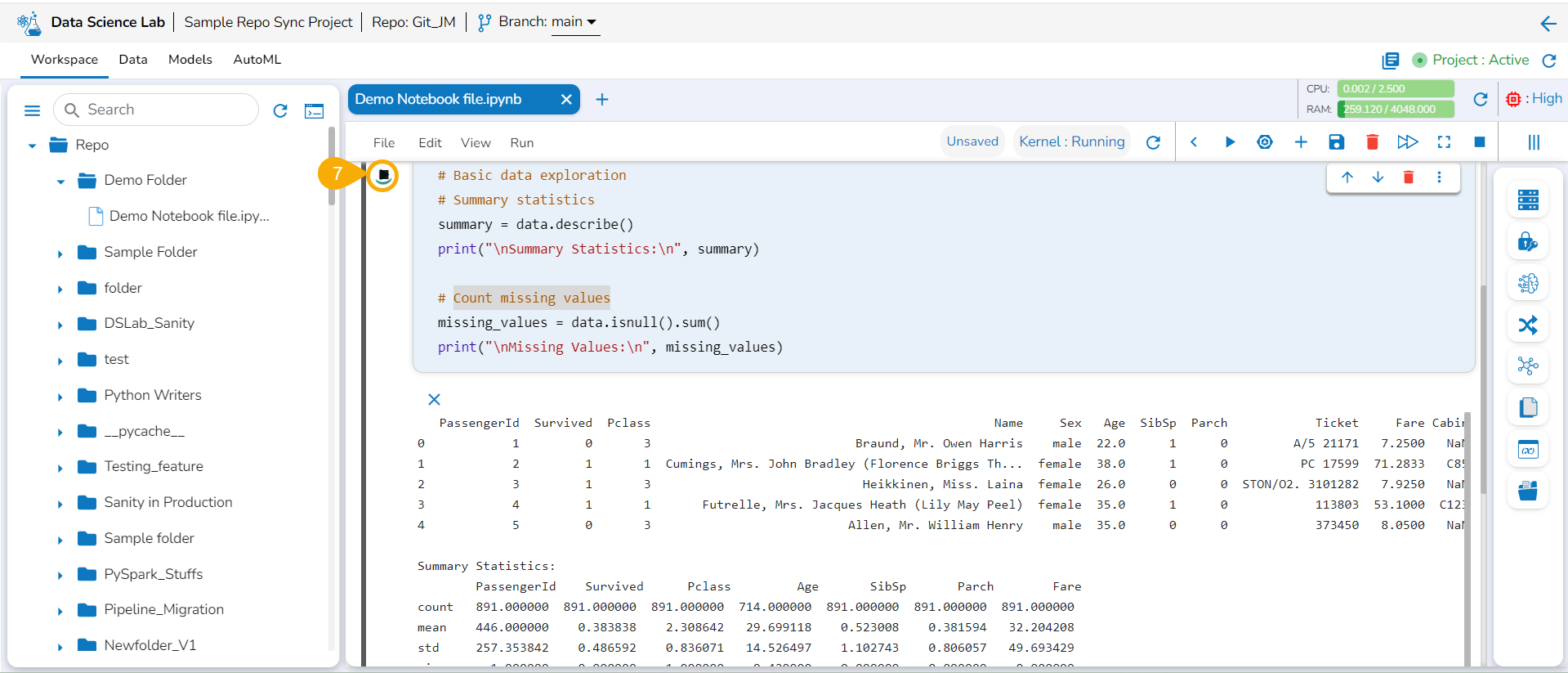
Please Note: The Code cells also get code from the selected Notebook operations by using the right-side panel and selecting a specific option. E.g., The user can use the Data tab to get an added data set to the code cell.
The Run cell button is changed into the Interrupt cell icon while running the code.
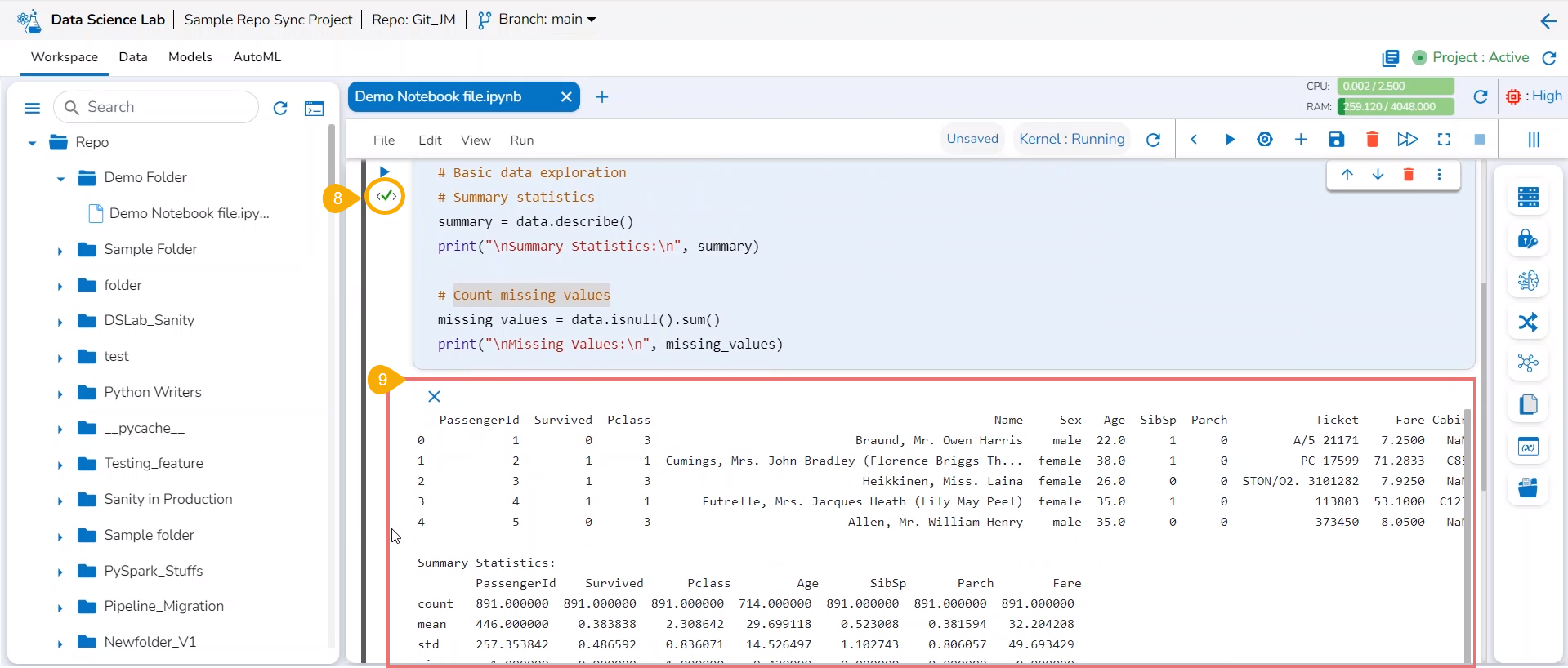
Once the code has run successfully a checkmark appears below the Run cell icon.
The code result is displayed below it.
Another code cell gets added below (as shown in the following image).
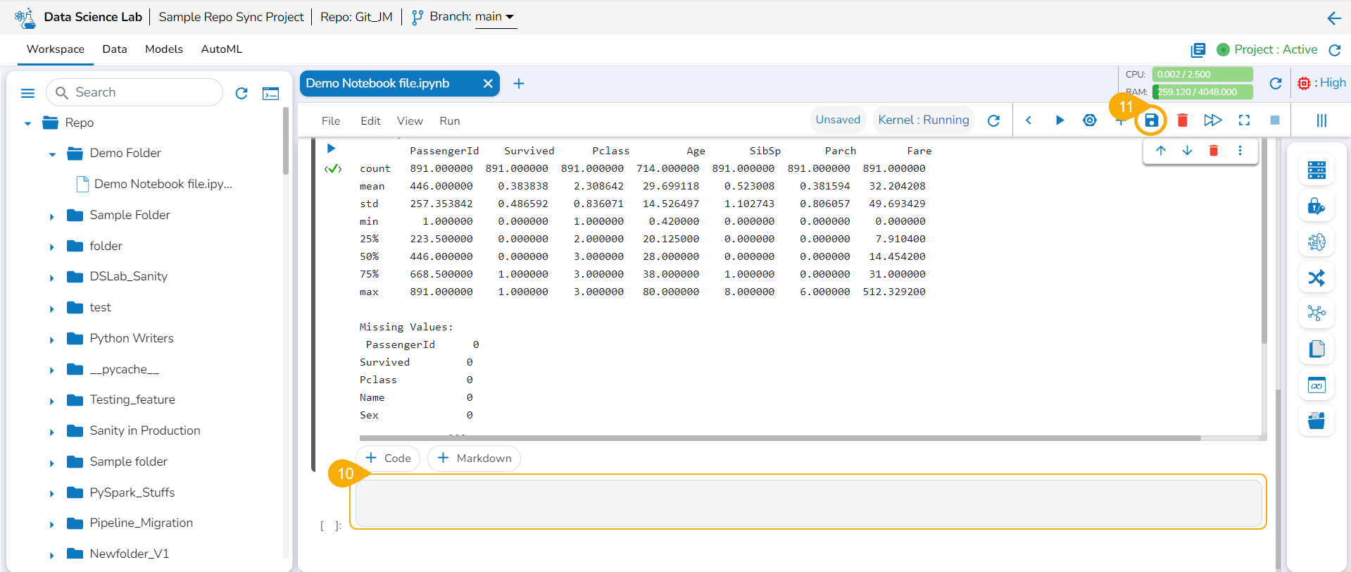
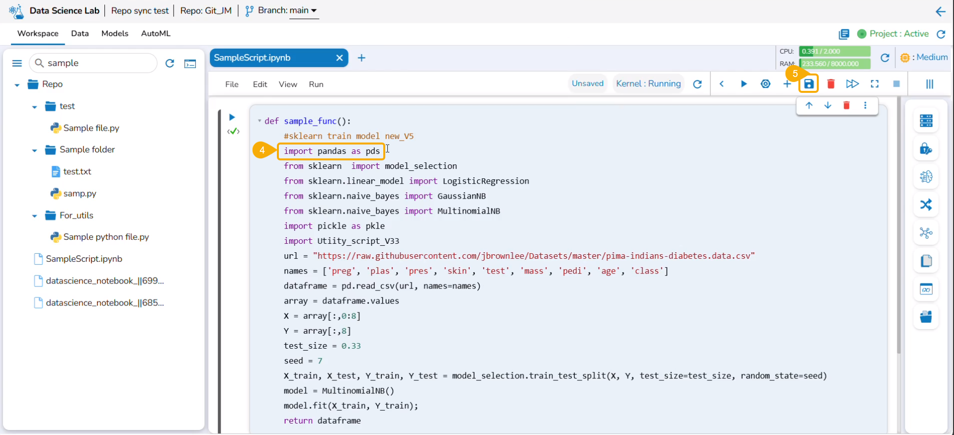
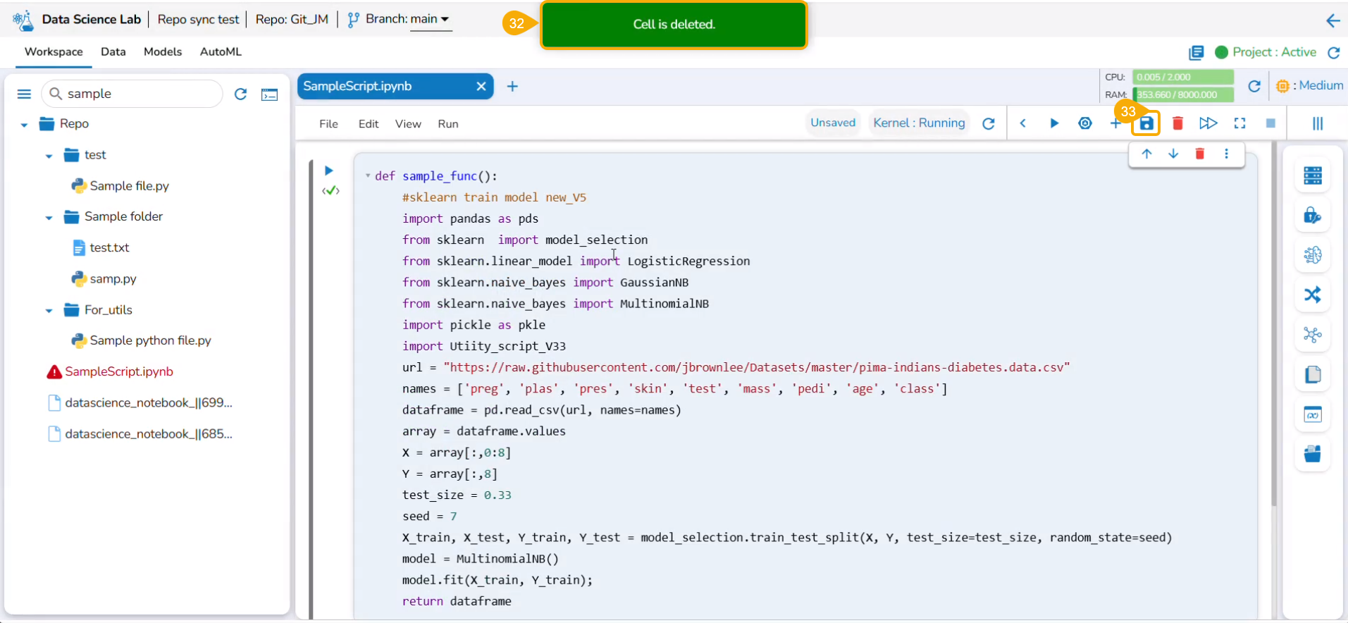
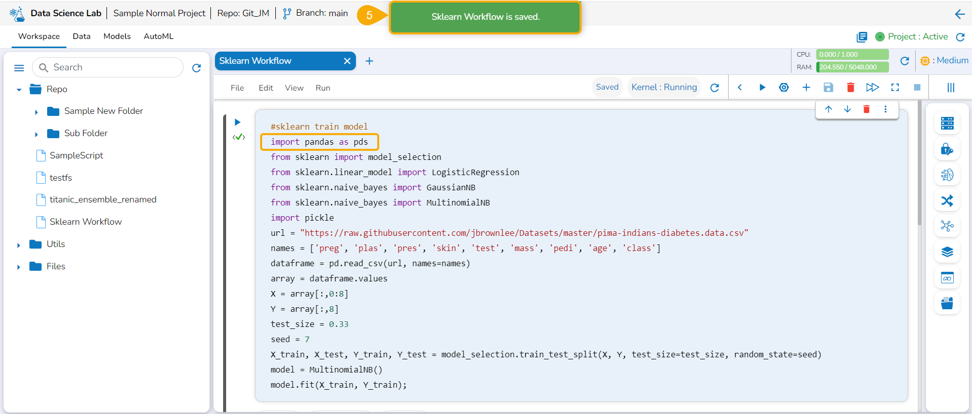
Click the Save icon provided for the Notebook.
A notification message appears to indicate the completion of the action.
The Data Science Notebook's status gets changed as saved and the new updates get saved in it.
Various Options provided to a Code Cell
By clicking on an inserted Code cell, some code-related options are displayed as shown in the image:
Sl. No.
Icon
Name
Action
1
Move the cell up
Moves the cell upwards
2
Please Note: The +Code,+Markdown, and +Assist options provided at the bottom of a cell insert a new cell after the given code/ Markdown cell.
The user should run the Notebook cells only after the Kernel is up and Running. If the user attempts to run a Notebook cell before the Kernel is started/ restarted, the following warning will be displayed.
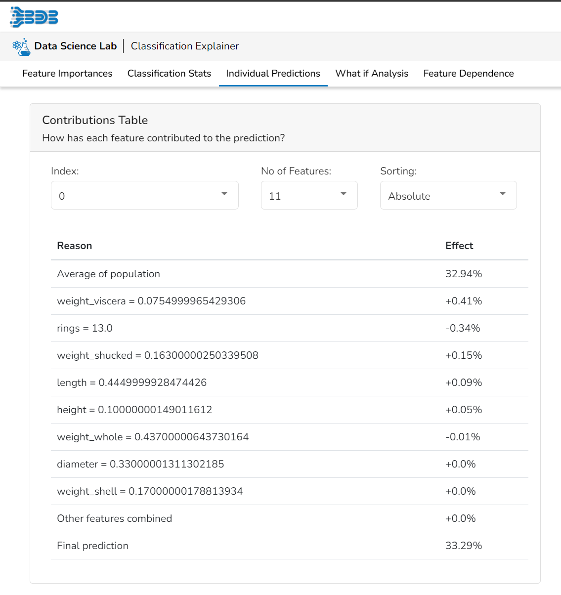
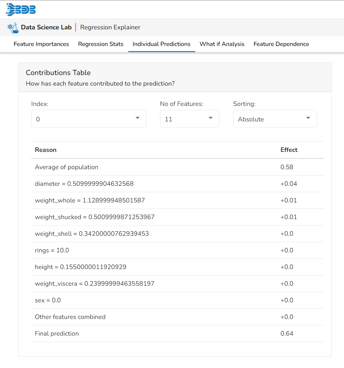
This table shows the contribution each feature has had on prediction for a specific observation. The contributions (starting from the population average) add up to the final prediction. This allows you to explain exactly how each prediction has been built up from all the individual ingredients in the model.
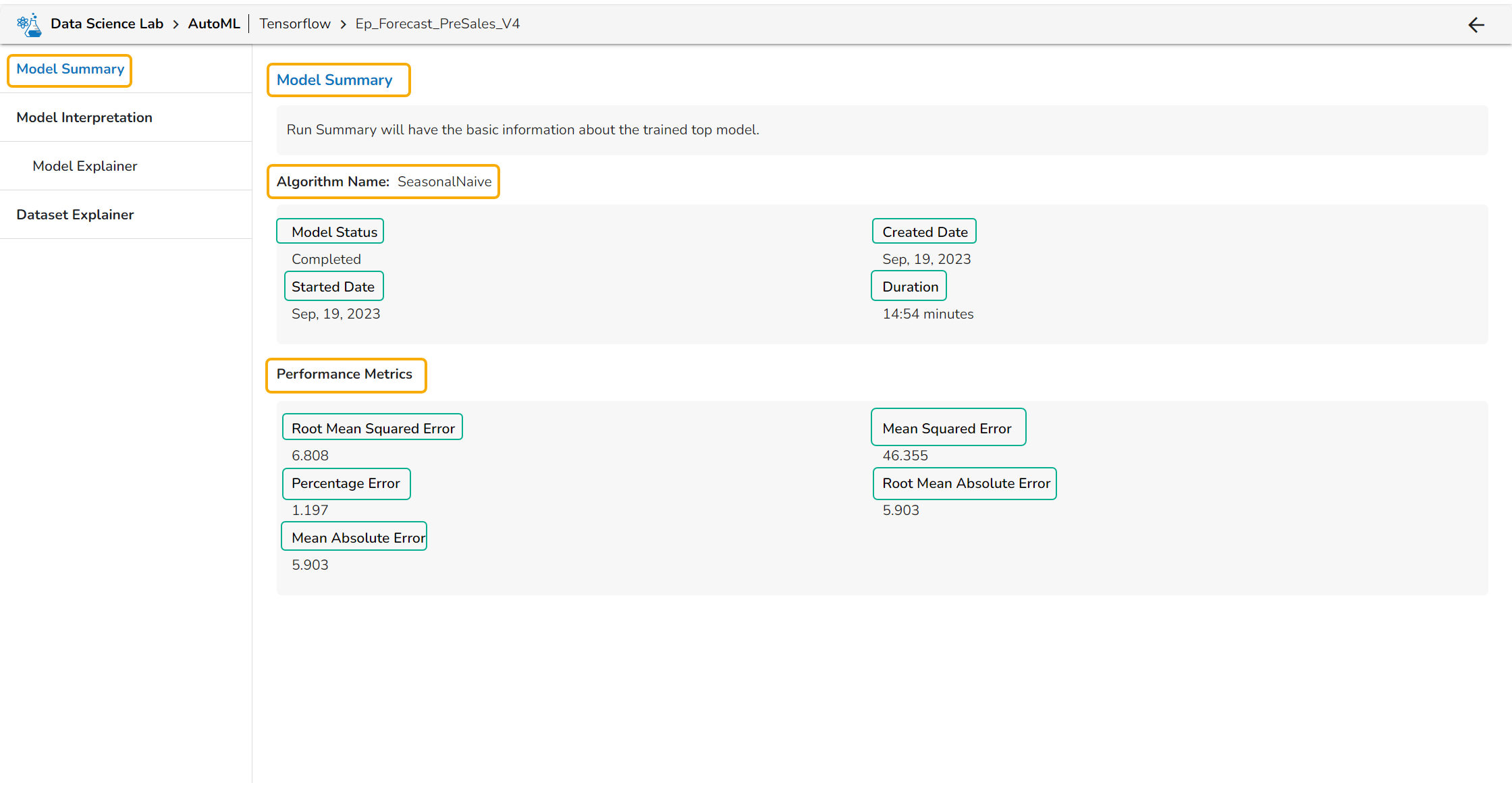
Regression Stats
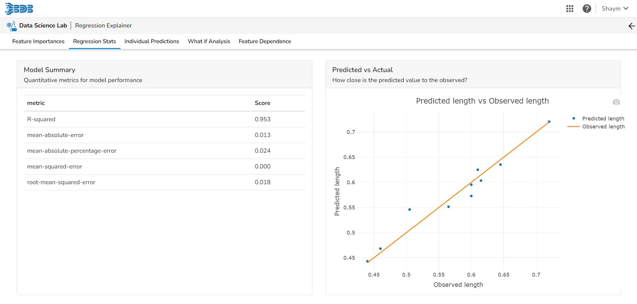
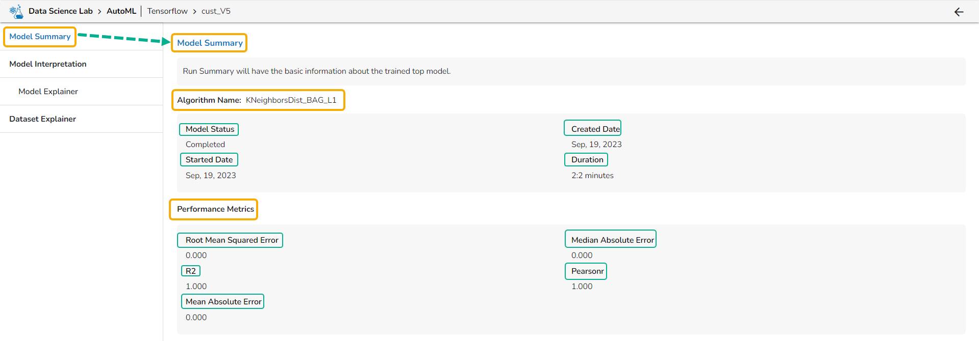
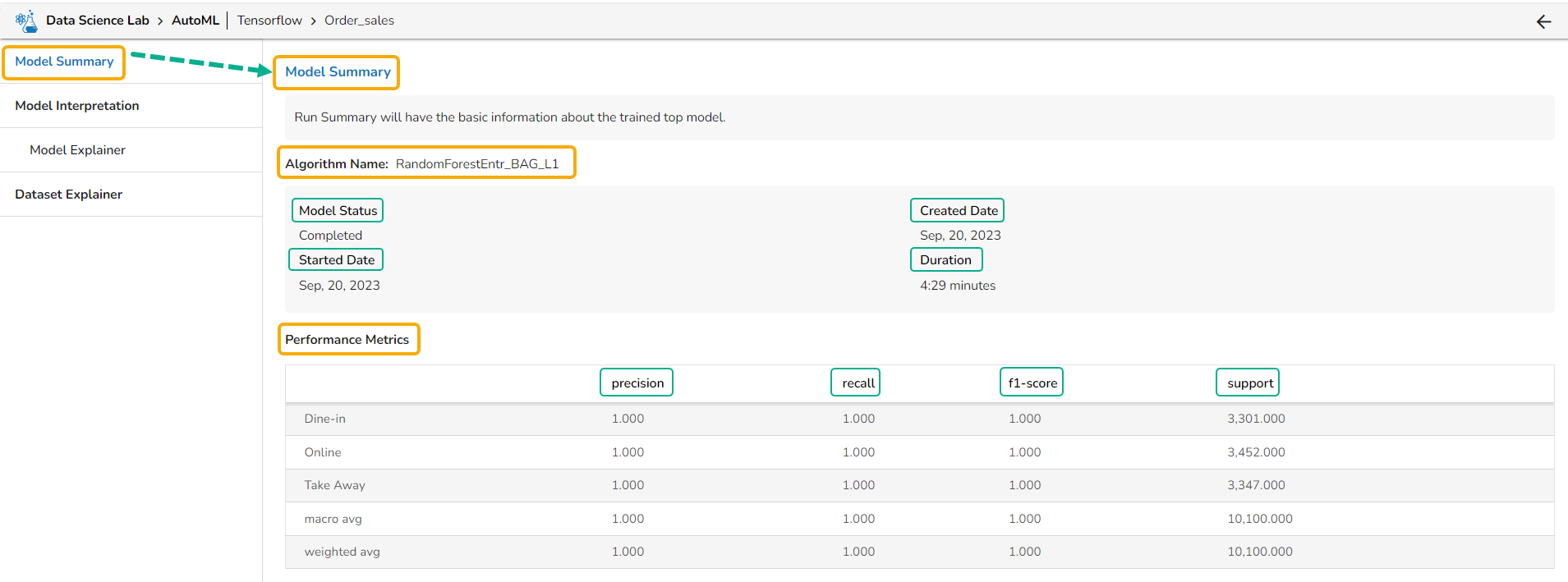
Model Summary
The user can find a number of regression performance metrics in this table that describe how well the model can predict the target column.
Predicted Vs Actual Plots
This plot shows the observed value of the target column and the predicted value of the target column. A perfect model would have all the points on the diagonal (predicted matches observed). The further away points are from the diagonal the worse the model is in predicting the target column.
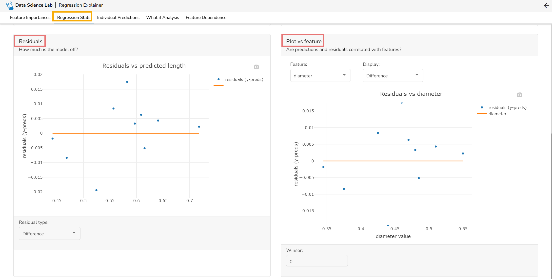
Residuals & Plot Vs Features
Residuals: The residuals are the difference between the observed target column value and the predicted target column value. in this plot, one can check if the residuals are higher or lower for higher /lower actual /predicted outcomes. So, one can check if the model works better or worse for different target value levels.
Plot vs Features: This plot displays either residuals (difference between observed target value and predicted target value) plotted against the values of different features or the observed or predicted target value. This allows one to inspect whether the model is more inappropriate for a particular range of feature values than others.
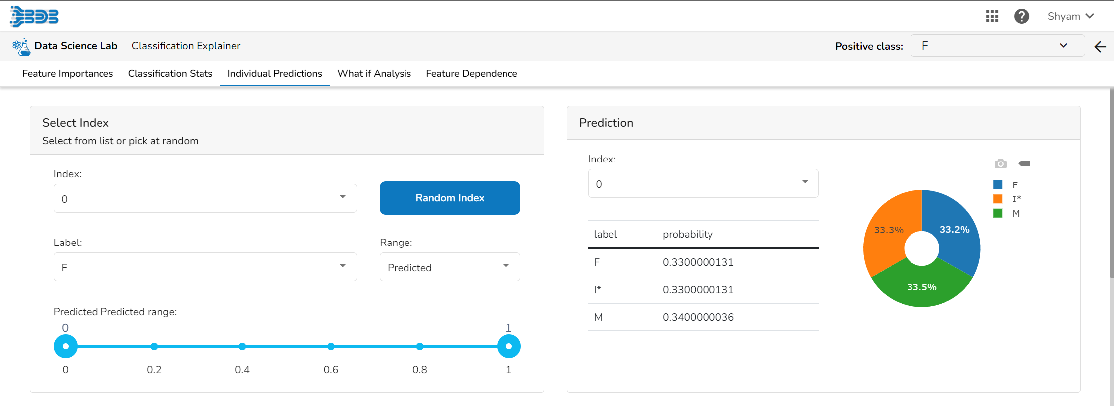
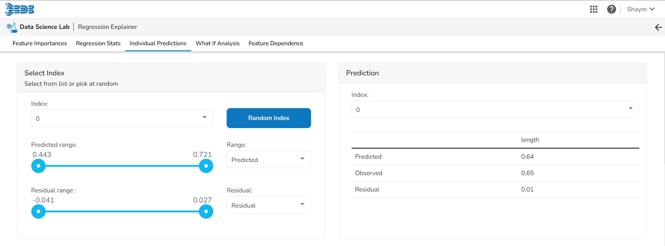
Individual Predictions
Select Index
The user can select a record directly by choosing it from the dropdown or hit the Random Index option to randomly select a record that fits the constraints. For example, the user can select a record where the observed target value is negative but the predicted probability of the target being positive is very high. This allows the user to sample only false positives or only false negatives.
Prediction
It displays the predicted probability for each target label.
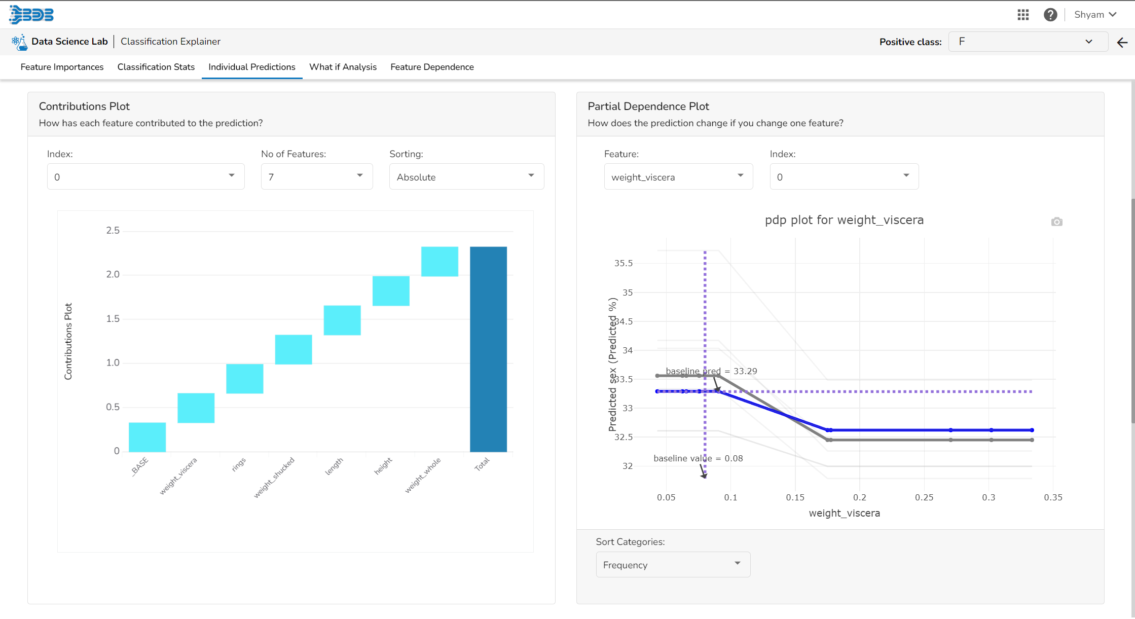
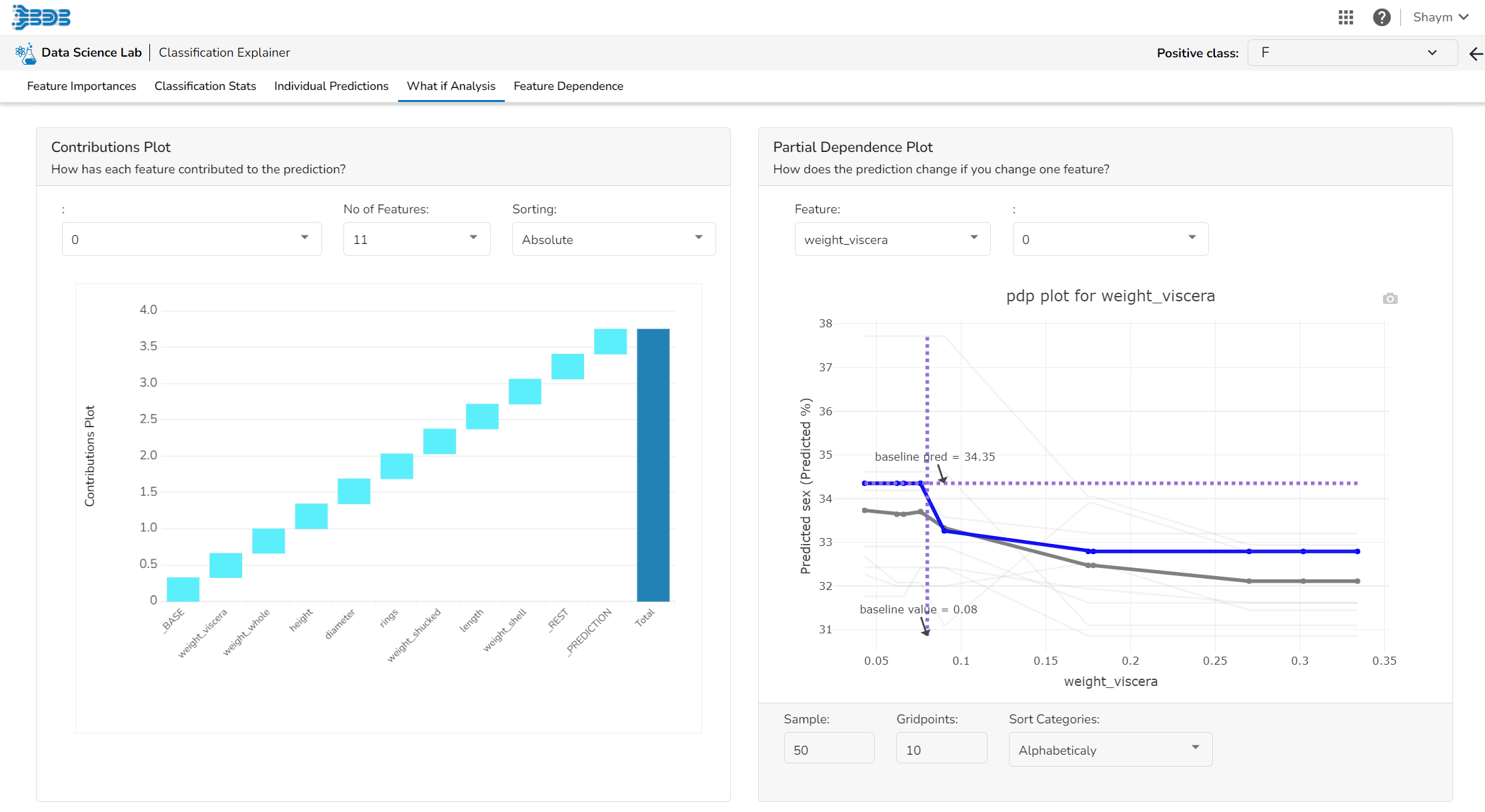
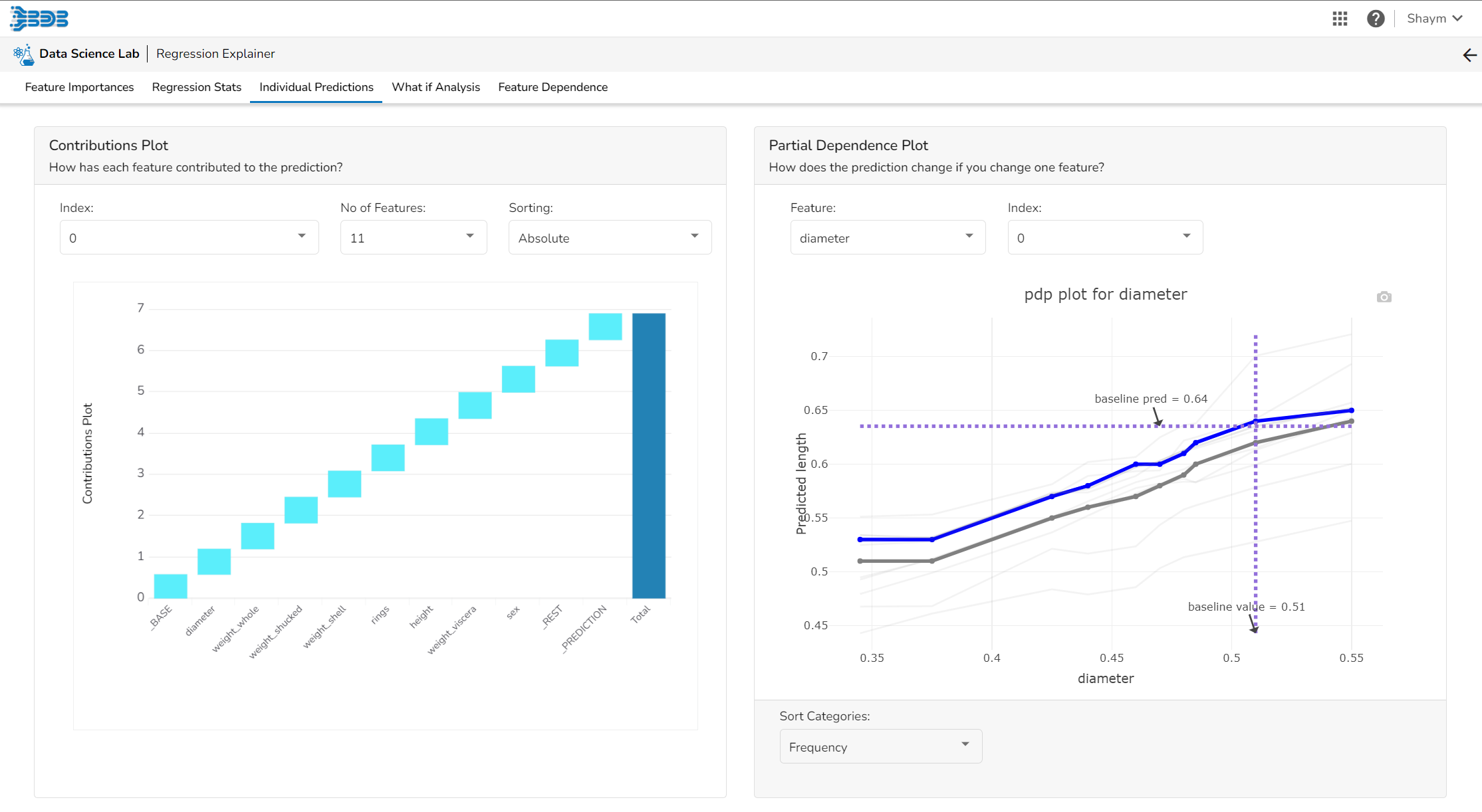
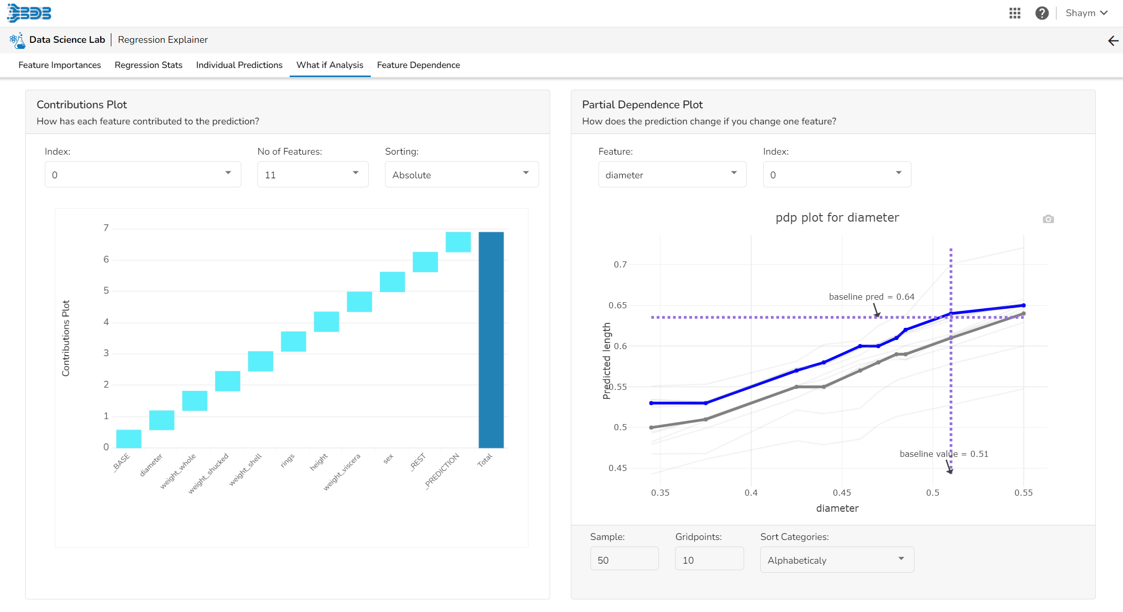
Contributions Plot
This plot shows the contribution that each feature has provided to the prediction for a specific observation. The contributions (starting from the population average) add up to the final prediction. This helps to explain exactly how each prediction has been built up from all the individual ingredients in the model.
Partial Dependence Plot
The PDP plot shows how the model prediction would change if you change one particular feature. the plot shows you a sample of observations and how these observations would change with this feature (gridlines). The average effect is shown in grey. The effect of changing the feature for a single record is shown in blue. The user can adjust how many observations to sample for the average, how many gridlines to show, and how many points along the x-axis to calculate model predictions for (grid points).
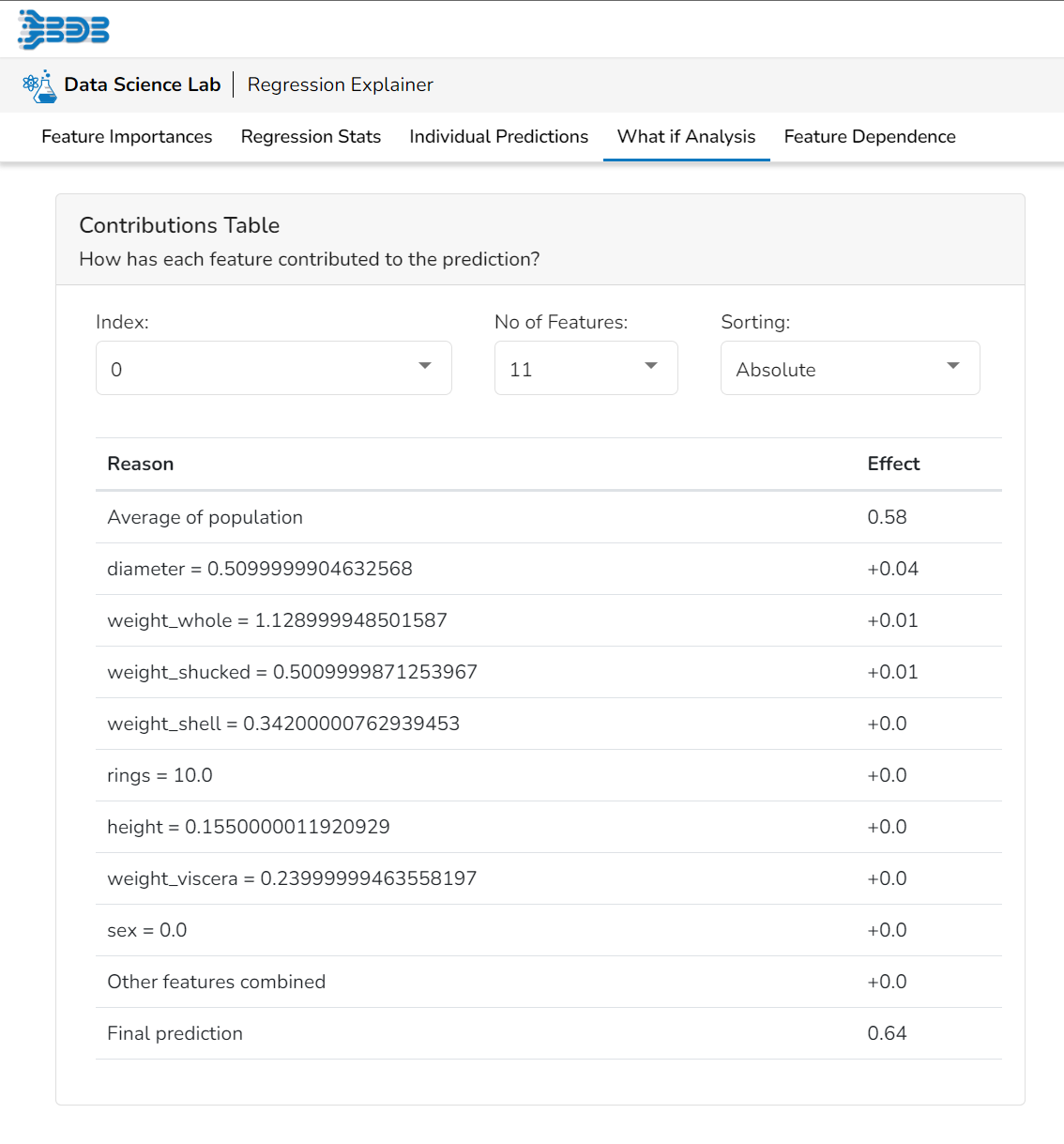
Contributions Table
This table shows the contribution each individual feature has had on the prediction for a specific observation. The contributions (starting from the population average) add up to the final prediction. This allows you to explain exactly how each individual prediction has been built up from all the individual ingredients in the model.
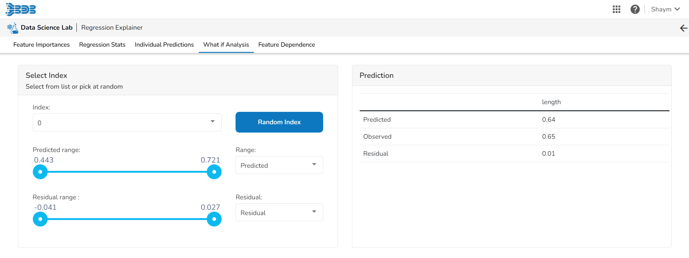
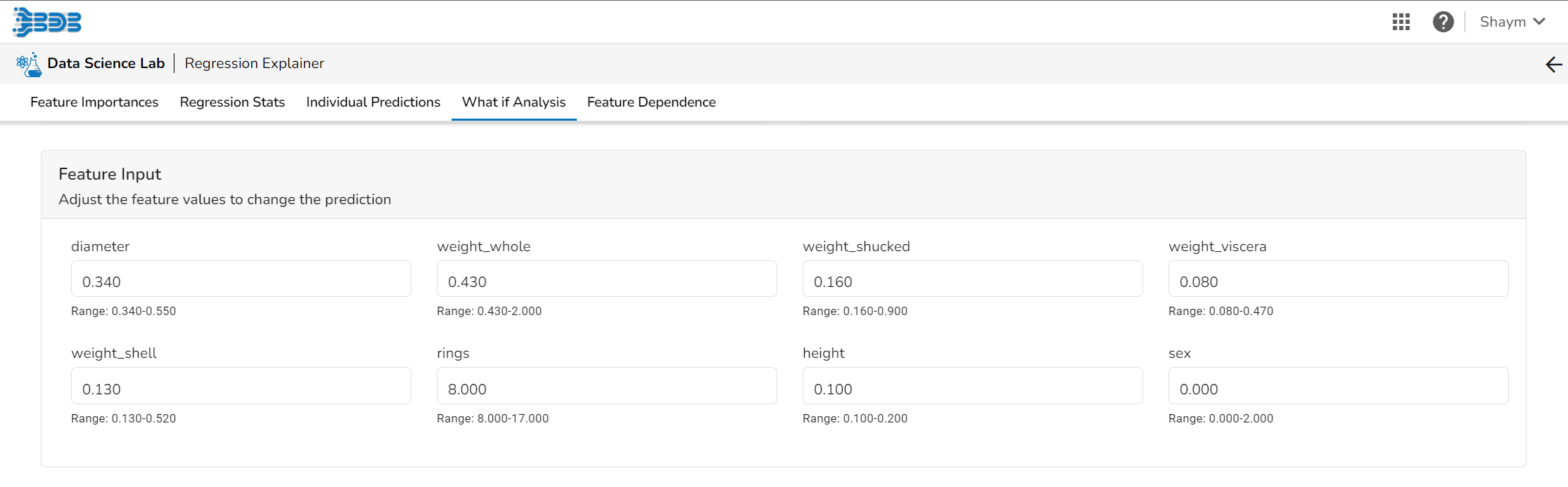
What If Analysis
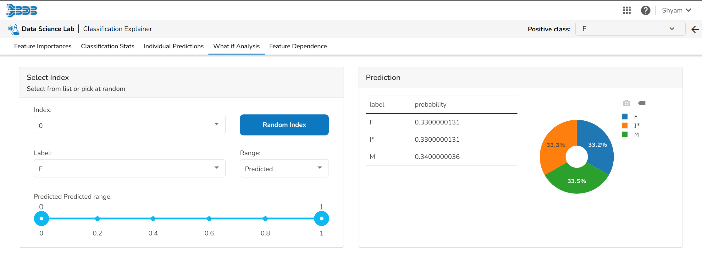
Select Index
The user can select a record directly by choosing it from the dropdown or hit the Random Index option to randomly select a record that fits the constraints. For example, the user can select a record where the observed target value is negative but the predicted probability of the target being positive is very high. This allows the user to sample only false positives or only false negatives.
Prediction
It displays the predicted probability for each target label.
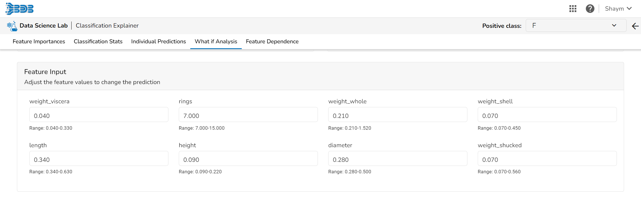
Feature Input
The user can adjust the input values to see predictions for what-if scenarios.
Contribution & Partial Dependence Plots
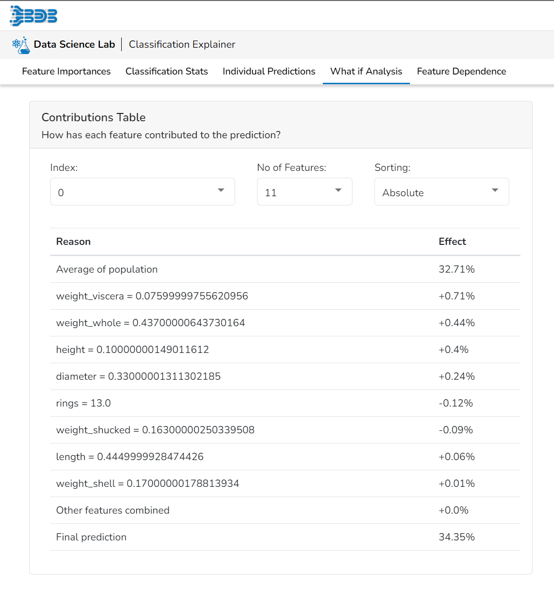
Contributions Table
This table shows the contribution each individual feature has had on the prediction for a specific observation. The contributions (starting from the population average) add up to the final prediction. This allows you to explain exactly how each individual prediction has been built up from all the individual ingredients in the model.
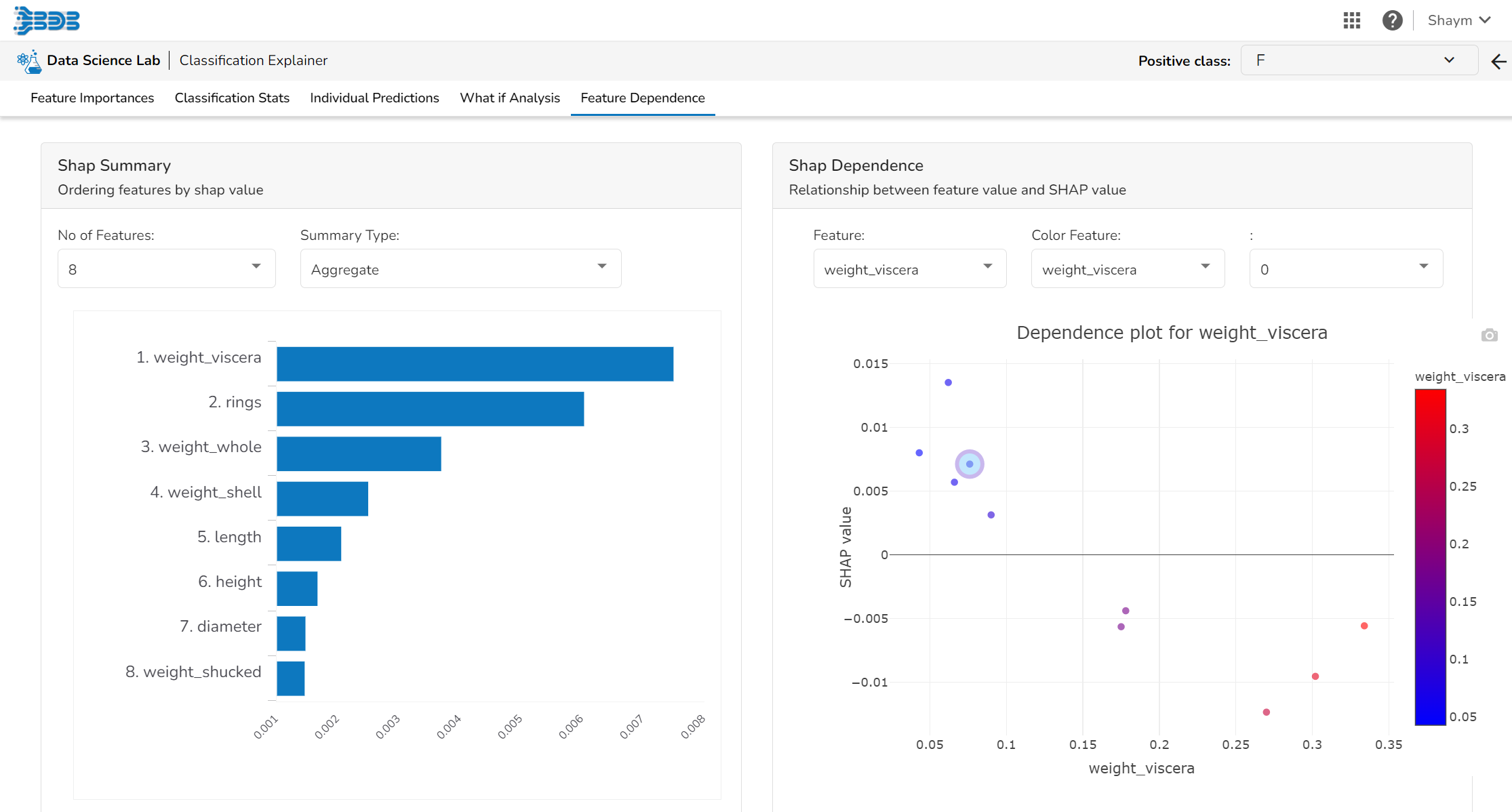
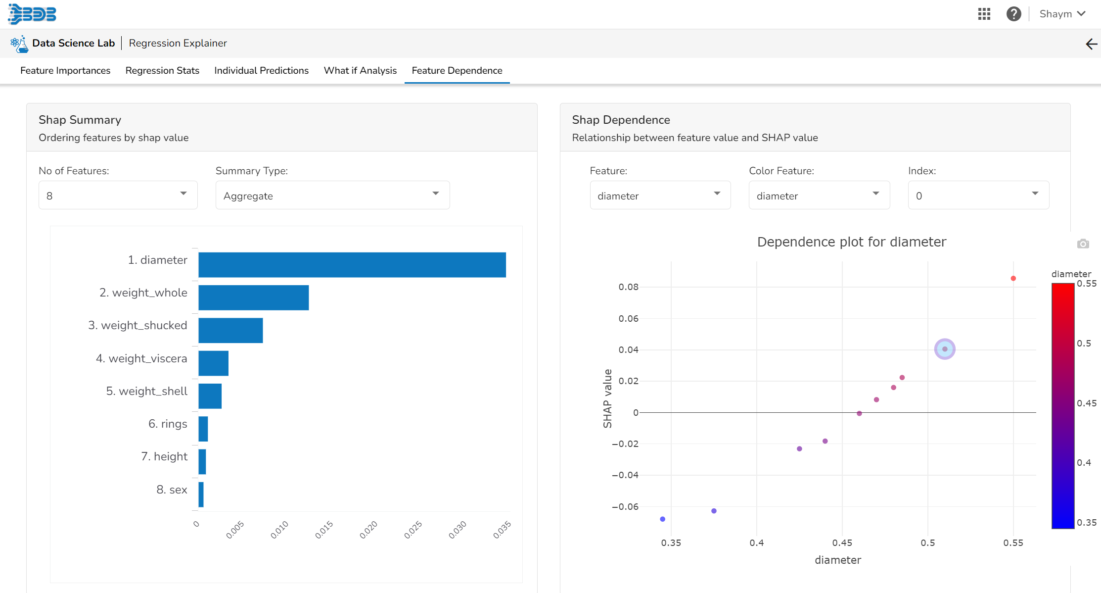
Feature Dependence
Shap Summary
The Shap Summarysummarizes the Shap values per feature. The user can either select an aggregate display that shows the mean absolute Shap value per feature or get a more detailed look at the spread of Shap values per feature and how they co-relate the feature value (red is high).
Shap Dependence
This plot displays the relation between feature values and Shap values. This allows you to investigate the general relationship between feature value and impact on the prediction. The users can check whether the model uses features in line with their intuitions, or use the plots to learn about the relationships that the model has learned between the input features and the predicted outcome.
This page provides model explainer dashboards for Classification Models.
Check out the given walk-through to understand the Model Explainer dashboard for the Classification models.
Feature Importance
This table shows the contribution each feature has had on prediction for a specific observation. The contributions (starting from the population average) add up to the final prediction. This allows you to explain exactly how each prediction has been built up from all the individual ingredients in the model.
Classification Stats
This tab provides various stats regarding the Classification model.
It includes the following information:
Global cutoff
Select a model cutoff such that all predicted probabilities higher than the cutoff will be labeled positive and all predicted probabilities lower than the cutoff will be labeled negative. The user can also set the cutoff as a percentile of all observations. By setting the cutoff it will automatically set the cutoff in the multiple other connected components.
Model Performance Metrics
It displays a list of various performance metrics.
Confusion Matrix
The Confusion matrix/ shows the number of true negatives (predicted negative, observed negative), true positives (predicted positive, observed positive), false negatives (predicted negative but observed positive), and false positives (predicted positive but observed negative). The number of false negatives and false positives determine the costs of deploying an imperfect model. For different cut-offs, the user will get a different number of false positives and false negatives. This plot can help you select the optimal cutoff.
Precision Plot
The user can see the relation between the predicted probability that a record belongs to the positive class and the percentage of observed records in the positive class on this plot. The observations get binned together in groups of roughly equal predicted probabilities and the percentage of positives is calculated for each bin. a perfectly calibrated model would show a straight line from the bottom left corner to the top right corner. a strong model would classify most observations correctly and close to 0% or 100% probability.
Classification Plot
This plot displays the fraction of each class above and below the cut-off.
ROC AUC Plot
The ROC curve is created by plotting the true positive rate (TPR) against the false positive rate (FPR) at different classification thresholds.
The true positive rate is the proportion of actual positive samples that are correctly identified as positive by the model, i.e., TP / (TP + FN). The false positive rate is the proportion of actual negative samples that are incorrectly identified as positive by the model, i.e., FP / (FP + TN).
PR AUC Plot
It shows the trade-off between Precision and Recall in one plot.
Lift Curve
The Lift Curve chart shows you the percentage of positive classes when you only select observations with a score above the cut-off vs selecting observations randomly. This displays to the user how much it is better than the random (the lift).
Cumulative Precision
This plot shows the percentage of each label that you can expect when you only sample the top x% with the highest scores.
Individual Predictions
Select Index
The user can select a record directly by choosing it from the dropdown or hit the Random Index option to randomly select a record that fits the constraints. For example, the user can select a record where the observed target value is negative but the predicted probability of the target being positive is very high. This allows the user to sample only false positives or only false negatives.
Prediction
It displays the predicted probability for each target label.
Contributions Plot
This plot shows the contribution that each feature has provided to the prediction for a specific observation. The contributions (starting from the population average) add up to the final prediction. This helps to explain exactly how each prediction has been built up from all the individual ingredients in the model.
Partial Dependence Plot
The PDP plot shows how the model prediction would change if you change one particular feature. the plot shows you a sample of observations and how these observations would change with this feature (gridlines). The average effect is shown in grey. The effect of changing the feature for a single record is shown in blue. The user can adjust how many observations to sample for the average, how many gridlines to show, and how many points along the x-axis to calculate model predictions for (grid points).
Contributions Table
This table shows the contribution each individual feature has had on the prediction for a specific observation. The contributions (starting from the population average) add up to the final prediction. This allows you to explain exactly how each individual prediction has been built up from all the individual ingredients in the model.
What If Analysis
The What If Analysis is often used to help stakeholders understand the potential consequences of different scenarios or decisions. This tab displays how the outcome would change when the values of the selected variables get changed. This allows stakeholders to see how sensitive the outcome is to different inputs and can help them identify which variables are most important to focus on.
What-if analysis charts can be used in a variety of contexts, from financial modeling to marketing analysis to supply chain optimization. They are particularly useful when dealing with complex systems where it is difficult to predict the exact impact of different variables. By exploring a range of scenarios, analysts can gain a better understanding of the potential outcomes and make more informed decisions.
Select Index & Prediction
Feature Input
The user can adjust the input values to see predictions for what-if scenarios.
Contribution & Partial Dependence Plots
In a What-if analysis chart, analysts typically start by specifying a baseline scenario, which represents the current state of affairs. They then identify one or more variables that are likely to have a significant impact on the outcome of interest, and specify a range of possible values for each of these variables.
Contributions Table
This table shows the contribution each individual feature has had on the prediction for a specific observation. The contributions (starting from the population average) add up to the final prediction. This allows you to explain exactly how each individual prediction has been built up from all the individual ingredients in the model.
Feature Dependence
Shap Summary
The Shap Summary summarizes the Shap values per feature. The user can either select an aggregate display that shows the mean absolute Shap value per feature or get a more detailed look at the spread of Shap values per feature and how they co-relate the feature value (red is high).
Shap Dependence
This plot displays the relation between feature values and Shap values. This allows you to investigate the general relationship between feature value and impact on the prediction. The users can check whether the model uses features in line with their intuitions, or use the plots to learn about the relationships that the model has learned between the input features and the predicted outcome.
Actions Icons from Header
This page covers all the actions provided for a Data Science Notebook file.
The Notebook Action icons (as provided below) help to apply various actions to the code/ code cell when clicked. They are provided on the top right side of the Data Science Notebook page.
The table given below lists all the Actions available in the Notebook Menu Bar:
Icon
Icon Name
Action
/
Please Note: The Actions icons will be disabled for other file types under a Repo Sync Project.
Share a Model
The share option for a model facilitates the user to share it with other users and user groups. It also helps the user to exclude the privileges of a previously shared model.
Sharing a Model
Check out the following video for guidance on the Share model functionality.
Create Project
This page explains project creation steps for a Data Science Lab Project.
What is a Project?
A Data Science Project created inside the Data Science Lab is like a Workspace inside which the user can create and store multiple data science experiments and their associated artifacts.
Forecasting Model Explainer
Saving Artifacts using a DS Notebook
Linter functionality in use for a Repo Sync Project
Deleting a Model
Adjustable Repository Panel
Accessing and Modifying the Default Project Settings
Expanding and Collapsing Markdown Cells
Assigning Verious Levels to Markdown Cells
Navigate to the Models tab where your saved models are listed.
Find the Model you want to share and select it.
Click the Share icon for that model from the Actions column.
The Manage Access page opens for the selected model.
Select permissions using the Grant Permissions checkboxes.
Navigate to the Users or User tab to select user(s) or user group(s).
Use the search function to locate a specific user or user group you want to share the Model with.
Select a user or user group using the checkbox.
Click the Save option.
Manage Access page for the selected Model
A notification message appears ensuring that it has been shared.
The selected user/ user group will be listed under the Granted Permissions section.
Accessing a Shared Model
Log in to the user account where the Model has been shared.
Navigate to the Projects page within the DS Lab module.
The Project where the source model was created will be listed.
Click the View icon to open the shared Project.
Open the Model tab for the project.
Locate the Shared Model, which will be marked as shared, in the Model list.
Shared Model with View Permission
When a Model is shared from User A to User B with View Permission, User B will have the following privileges:
View the shared model.
Shared Model with Edit Permission
When a Model is shared from User A to User B with Edit Permission, User B will have the following privileges:
View the model and trigger the explainer dashboard job.
View the model and generate the explainer dashboard.
View the model and migrate.
Shared Model with Execute Permission
When a Model is shared from User A to User B with Execute Permission, User B will have the following privileges:
View the model and Register the Model into the Data Pipeline.
View the model, Update and save the model information, and Register the model as API.
View the model and unregister the registered model as an API service.
Please Note: A targeted share user cannotre-share or delete a shared modelregardless of the permission level (View/ Edit/Execute).
Excluding Users
Check out the illustration on using the Exclude Users functionality.
Navigate to the Models tab.
Select a model from the displayed list.
Click the Share icon.
The Manage Access window appears for the selected model.
Select permissions using the checkboxes from the Grant Permissions option.
Open the User Groups tab.
Select user group(s) using the checkbox(es).
Navigate to the Exclude Users tab.
Select users to be excluded using checkboxes.
Click the Save option.
A notification message appears.
The excluded users will be listed under the Excluded Users section.
Including an Excluded User
Check out the illustration for including an excluded user to access a shared model.
Navigate to the Manage Access window for a shared model.
The Excluded Users section will list the excluded users from accessing that model.
Select a user from the list.
Click the Include User icon.
The Include User dialog box opens.
Click the Yes option.
A notification message appears ensuring that the selected user is included.
The user gets removed from the Excluded Users section.
Revoking Privileges
Check out the illustration on revoking privileges for a user.
Navigate to the Manage Access window for a shared model.
The Granted Permissions section will list the shared user(s)/ user group(s).
Select a user/ user group from the list.
Click the Revoke icon.
The Revoke Privileges dialog box opens.
Click the Yes option.
A notification message ensures that shared model privileges are revoked for the selected user/user group. The user/ user group will be removed from the Granted Permissions section.
Please Note: The same set of steps can be followed to revoke privileges for a user group.
Creating a new Project
Check out the given illustration on how to create a DSL Project.
Pre-requisite:The users must have the following Admin-level settings configured to access and use the Repo Syncs Project functionality inside the DS Lab module.
Configuring the DS Lab Settings option is mandatory before beginning with the Data Science Project creation.
Also, select the Algorithms by using the Algorithms field from the DS Lab Settings section you wish to use for your DS Lab project.
The user must have the following settings done.
The token key has to be configured for the DS Lab module.
The repository and branch have to be specified to save the settings.
The user must complete the following :
Token key – bdbvcstoken
User id key - bdbvcsuserid
The user must do the following User-level configuration to create a Repo Sync DS Lab project.
Steps to create a new DSL Project
Navigate to the Home page of the Data Science Lab module.
Click the Create icon from the homepage.
The Create Project or Feature Store drawer opens.
Click the Create option provided for the Project.
The Create Project opens to provide the related information for a new Project.
Provide the following details for a new project:
Project Name: Give a name to the new project.
Project Description: Describe the project.
Select Algorithms: Select algorithms using the drop-down menu.
Environment: Allows users to select the environment they want to work in. Currently, supported environments are PythonTensorFlow, Python PyTorch, and PySpak.
Users who select the TensorFlow environment do not need to install packages like the TensorFlow and Keras explicitly in the notebook. These packages can be imported inside the notebook.
Users who select the
Resource Allocation: This allows the users to allocate CPU/ GPU and memory to be used by the Notebook container inside a given project. The currently supported Resource Allocation options are Low, Medium, and High.
Idle Shutdown: It allows the users to specify the idle time limit after which the notebook session will get disconnected, and the project will be deactivated. To use the notebook again, the project should be activated. The supported Idle Shutdown options are 30m, 1h, and 2h.
External Libraries: Mention the names of external libraries (if a specific version is required then mention the library name with the version number) that must be installed in your DSL project /notebook. The names of the external libraries should be separated only by commas (without space) for this field. This is an optional field.
After you fill in the mandatory fields the following modifiable fields appear with pre-selected values:
Image Name
Image Version
GPU Type: Select GPU type from the drop-down menu (Currently we support Nvidia as the GPU Type).
GPU Limit: Set the GPU limit using this field (This field appears only after the GPU Type option is selected).
Nodepool: Use this field to select a node pool option for the efficient execution of your data science project.
Sync git repo at project creation: Put a checkmark in the given checkbox to avail of sync git repo while creating a DS Lab project.
Please Note:
You can enable the Sync git repo at the project creation option to make your DSL Project a Git Repo Sync Project. The Repo Sync Projects will be displayed in the Project list with a branch icon in their title.
You can configure the Git access for a normal Data Science Lab project by configuring the Git Repository and Git Branch fields while creating a new project. Such projects will display the branch icon without the drop-down option while opening that project. For example,
Click the Saveoption.
The Create Project Drawer
The confirmation message appears.
The newly created project gets saved, and it appears on the screen.
The newly created Project gets added at the top of the Projects list
Move the cell down
Moves the cell downwards
3
Delete Cell
Deletes the code cell.
4
More Actions
Opens four more actions that include:
Transform, Save Model, Predict, and Save artifact.
Expand / Collapse
Expands or collapses the Actions Menu Bar.
Run Current cell
Runs code given for a specific cell.
Linter
Opens the Linter panel.
Add Pre cell
Adds a code cell before the first cell.
Save
Saves the Notebook updates.
Delete cell
Removes the selected cell.
Restart kernel
Restarts the kernel by killing the current session and creates a new session.
Interrupt cell
Interrupts the running cell
Logs
Opens Logs window to display logs.
Undo Delete cell
Reverts the Deleted cell.
Cut cell
Cuts the code from a specific cell.
Copy cell
Copies the code from a specific cell.
Paste cell
Pastes the cut or copied code to the selected cell.
/
Auto Save
Auto-saves the Notebook updates when enabled.
Run all cells
Runs the codes for all the cells.
Shutdown
Stops the Kernel/Disconnects the instance and allocated resources.
Git Console
Git Console functionality helps the data scientists apply various Git commands to their Notebook scripts inside the Repo Sync projects.
Check out the illustration on using the Git Console option inside the Data Science Lab repo sync projects.
Using Git Console
Navigate to the Workspace tab of an activated Repo Sync Project.
Select a .ipynb file from the Repo Sync Project.
The file content opens.
Edit the displayed script.
Click the Save icon.
A notification ensures that the script is saved with the recent changes.
Open the same script in the Git repository.
Click the Edit option and access the script in the editable format.
Click the Commit changes option.
The Commit changes dialog box opens.
Provide a commit message.
Choose a checkbox to select how the changes should be committed.
The script in the Git repository will be modified.
Navigate to the Workspace tab of the Notebook and click the Git Consol icon.
The Git Console panel opens where you can put the Git command to be performed on the selected script.
Use the Resize panel icon to resize the Git Console panel.
Use git status command to reflect the changes.
The next commands that can be used are git add and git commit to acknowledge new changes in the file.
The git commit command generates the information inside the panel about the new changes.
The git push command is used to push the new changes to the Git Repository. The git push command has been rejected since there is a change in the repository version of the same file and the console suggests using the git pull command.
The git pull command has been used to pull the distant changes from the repository.
At the end of the git pull command, it is hinted to use git config pull rebase false as a default strategy.
The git config pull rebase false command is committed.
The auto merge failed due to the merge conflict in the selected file.
Navigate to the Workspace tab.
The file title appears in red to indicate the conflict.
The cells containing conflicted content are highlighted in the script.
Click the Delete icon for the conflicted cells.
The Delete Cell window appears.
Click the Yes option.
A notification message appears to ensure that the conflicted cell is removed from the script.
Click the Save icon for the script.
Please Note: The user must resolve all the conflicts in the selected file, before saving it.
A notification ensures that the script is saved.
The saved script reflects the remote changes.
The color of the selected file title also gets changed.
By hovering on the file name, it displays the current status of the file. For example, the given image shows that for the current file conflicts are resolved, but it is in uncommitted status.
Please Note: the user can click the Refresh icon to refresh the status of the file.
Click the GitConsole icon.
The Git Console space gets displayed.
The Git commands used in the example are git add, git commit, and git push.
Navigate to the script saved remotely (in the Git repository).
The script displays the recent changes committed using the Git Console space for a Repo Sync Project.
Commonly used Git Commands
All the Git commands will be supported in the Git Console. Please find some of the commonly used Git commands listed below.
Import Model
External models can be imported into the Data Science Lab and experimented inside the Notebooks using the Import Model functionality.
Please Note:
The External models can be registered to the Data Pipeline module and inferred using the Data Science Lab script runner.
Only the Native prediction functionality will work for the External models.
Importing a Model
Check out the illustration on importing a model.
Navigate to the Model tab for a Data Science Project.
Click the Import Model option.
The user gets redirected to upload the model file. Select and upload the file.
A notification message appears.
The imported model gets added to the model list.
Please Note: The imported models are referred to as External models in the model list and are marked with a prefix to their names (as displayed in the above-given image).
Exporting a Model to the Data Pipeline
You can integrate and export cutting-edge Data Science models into your data pipeline, ensuring optimized performance, real-time insights, and data-driven decision-making. The user needs to start a new .ipynb file with a wrapper function that includes Data, Imported Model, Predict function, and output Dataset with predictions.
Navigate to a Data Science Notebook (.ipynb file) from an activated project. In this case, a notebook has been imported with the wrapper function.
Access the Imported Model inside this .ipynb file.
Load the imported model to the Notebook cell.
Mention the loaded model in the inference script.
Run the code cell with the inference script.
The Data preview is displayed below.
Click the Register option for the imported model from the ellipsis context menu.
The Register Model dialog box appears to confirm the model registration.
Click the Yes option.
A notification message appears, and the model gets registered.
Export the script using the Export functionality provided for the Data Science Notebook (.ipynb file).
Another notification appears to ensure that the Notebook is saved.
The Export to Pipeline window appears.
Select a specific script from the Notebook. or Choose the Select All option to select the full script.
Select the Next option.
Click the Validate icon to validate the script.
A notification message appears to ensure the validity of the script.
Click the Export to Pipeline option.
A notification message appears to ensure that the selected Notebook has been exported.
Please Note: The imported model gets registered to the Data Pipeline module as a script.
Accessing the Exported Model within the Pipeline User interface
Navigate to the Data Pipeline Workflow editor.
Drag the DS Lab Runner component and configure the Basic Information.
Open the Meta Information tab of the DS Lab Runner component.
The user can connect the DS Lab Script Runner component to an Input Event.
Run the Pipeline.
The model predictions can be generated in the Preview tab of the connected Input Event.
Please Note:
The Imported Models can be accessed through the Script Runner component inside the Data Pipeline module.
Try out the Import Model Functionality yourself
Some of the Sample models and related scripts are provided below for the users to try this functionality. Please download them with a click, and use them inside your Data Science Notebook by following the above-mentioned steps.
Sample files for Sklearn
Sample files for Keras
Sample files for PyTorch
Notebook Version Control
This page explains the step by step process for Notebook migration and Push to VCS functionality.
Push into Git (Migration)
A Notebook script can be migrated across the space and server using the Push into GIT option.
Prerequisites: It is required to set the configuration for the Data Science Lab Migration using the Version Control option from the Admin module before migrating a DS Lab script or model.
Check out the walk-through on how to migrate/ export a Notebook script to the GIT Repository.
Select a Notebook from the Workspace tab.
Click the Ellipsis iconto get the Notebook list actions.
Click the Push into VCS option for the selected Notebook.
The Push into Git drawer opens.
Select the Git Export (Migration) option.
Provide a Commit Message in the given space.
The selected Notebook script version gets migrated to the Git Repository and the user gets notified by a message.
Importing a DSL Script from GIT
After exporting a DSL script, you can sign in to another user account on a different space or server and import the DSL script.
Click the Admin module from the Apps menu.
Select the GIT Migration option from the admin menu panel.
Click the Import File option.
The Import Document page opens, click the Import option as suggested in the following image.
The Migration- Document Import page opens.
Select New VCS as Version Control Configuration.
Select the DSLab option from the module drop-down menu.
Select a Notebook from the displayed list to open the available versions of that Notebook.
Select a Version that you wish to import.
Click the Migrate option.
A notification message appears informing that the file has been migrated.
Open the Data Science Lab module and navigate to the List Project Page.
The imported Notebook gets listed with the concerned DSL Project.
Please Note:
The user can migrate only the exported scripts (the exported scripts to the Data Pipeline).
While migrating a DSL Notebook/Script using the Export to Git functionality, the concerned Project under which the Notebook is created also gets migrated.
Version Control
Check out the illustrations on the Notebook Version Control functionality.
Select a Notebook file from the Workspace tab.
Open the Notebook file.
Modify the Notebook script.
Click the Save icon.
A message notifies the user that the workflow changes are saved.
Access the Context menu for the Notebook.
Click the Push into VCS option for the selected Notebook.
The Push into Version Controlling System drawer opens.
Select the Version Control option.
Provide a Commit Message.
The selected version of the Notebook gets pushed to VCS, and the same is informed by a message.
Open the context menu for the Notebook of which multiple versions are pushed to the VCS.
Click the Pull from VCS option from the Context menu.
The Pull from Version Controlling System drawer opens.
Select a version using the checkbox.
Click the Pull option.
A message appears to notify the user that the Notebook is pulled from the VCS.
Select the same Notebook file from the Repo folder of the Workspace tab, and open it
A message appears to notify that the selected workflow is started.
The user can verify the Notebook script will reflect the modifications done by the user for the pulled version of the Notebook.
Version control for a file Pulled from Git
The Version Control feature for a Notebook file pulled from Git differs from the Notebook file created/ owned by the user.
Click the Information option provided in the Context menu for a Notebook. It will mention Pulled from git if the selected Notebook is pulled from Git.
Please Note: The Notebook file from Git gets overwritten with each pull, consistently fetching the latest version and does not allow version selection.
Check out the illustration to understand the Version control steps for a Notebook file pulled from the Git Repo.
Writers inside a DS Notebook
File Folder Attributes
Adding a File to the File Folder
Adding a Folder to the File Folder
Unregistering a Model
Registering a Model
Data List Page
This section of the document describes the actions attributed to the added data inside a Data Science Lab project.
Preview
The Data Preview option displays a sample of the actual data for the user to understand the data values in a better way.
Navigate to the Dataset list inside a Project.
Share
This page describes the steps involved to share a Notebook script and access it as a shared Notebook.
Sharing a Notebook
The user can share a DSL Notebook across the teams using this feature.
Importing a Utility File
Restoring a Project
Deleting a Project Permanently
Saving and Loading a Data Science Model
Export as a Script to Pipeline
Model Explainer Genrator as a Job
Copy path functionality for a file stored inside the File Folder
Importing a file to the Files folder for a normal DS Project
Scheduling a Feature Store
Creating a Feature Store
PyTorch
environment do not need to install packages like
Torch
and
Torchvision
in the notebook. These packages can be imported inside the notebook.
Limit
Memory
Request (CPU)
Memory
Git Project: Select a project from the drop-down menu.
Git Branch: Select a branch option from the drop-down menu (The supported branches are main, migration, and version).
Sample python script based on the imported Pytorch model.
Click the Push option.
Select the Notebook option from the left side panel.
All the migrated Notebooks are listed. The user can use the Search bar to customize the displayed list of the exported Notebooks.
While migrating a DSL Notebook the utility files which are part of the same Project will also get migrated.
Click the Push option.
Pulled from git
Select either a Data Sandbox or Dataset from the displayed list.
Click the Preview icon for the selected data entity.
The Preview Data Sandbox or Preview Dataset page opens based on the selected data.
Preview of a Data Sandbox
Preview of a Dataset
Data Profile
This action helps users to visualize the detailed profile of data to know about data quality, structure, and consistency. A data profile is a summary of the characteristics of a dataset. It is created as a preliminary step in data analysis to better understand the data before performing an in-depth analysis.
Check out the illustration provided at the beginning to get the full view of the Data Profile page.
Navigate to the Data list page.
Select a Dataset from the list. It can be anything from a Dataset, Data Sandbox file, or Feature Store.
Click the Data Profile icon.
Accessing Data Profile icon
The Data Profile drawer opens displaying the Data Set information, Variable Types, Warnings, Variables, Correlation chart, missing values, and sample.
Displaying the Data Profile for the selected Data
Create Experiment
The users can create a supervised learning (Auto ML) experiment using the Create Experiment option.
Check out the illustration to create an auto ML experiment.
Navigate to the Dataset List page.
Select a Dataset from the list.
Click the Create Experiment icon.
Please Note: An experiment contains two steps:
Configure: Enter the Experiment name, Description, and Target column.
Select Experiment Type: Select an algorithm type from the drop-down menu.
A Classification experiment can be created for discrete data when the user wants to predict one of the several categories.
A Regression experiment can be created for continuous numeric values.
A Forecasting experiment can be created to predict future values based on historical data.
The Configure tab opens (by default) while opening the Create Experiment form.
Provide the following information:
Provide a name for the experiment.
Provide Description (optional).
Select a Target Column.
Select a Data Preparation from the drop-down menu.
Use the checkbox to select a Data Preparation from the displayed drop-down.
Select columns that need to be excluded from the experiment.
Use the checkbox to select a field to be excluded from the experiment.
Please Note: The selected fields will not be considered while training the Auto ML model experiment.
Selecting Columns to be excluded from the model training
Click the Next option.
Configure tab with selected Data Preparations and excluded fields
The user gets redirected to the Select Experiment Type tab.
Select a prediction model using the checkbox.
Based on the selected experiment type a validation notification message appears.
Click the Done option.
Selecting Experiment Type
A notification message appears.
The user gets redirected to the Auto ML list page.
The newly created experiment gets added to the list with the Status mentioned as Started.
Data Preparation
Data Preparation involves gathering, refining, and converting raw data into refined data. It is a critical step in data analysis and machine learning, as the quality and accuracy of the data used directly impact the accuracy and reliability of the results. The data preparation ensures that the data is accurate, complete, consistent, and relevant to the analysis. The data scientist can make more informed decisions, extract valuable insights, and unveil concealed trends and patterns within the raw data with the help of the Data Preparation option.
Navigate to the Data tab.
Select a Dataset from the list.
Click the Data Preparation icon.
The Preparation List window displays the preparation based on the selected Excel file. The user may use any of the displayed data preparation from the list.
The user can select a sheet name from the given drop-down menu.
Click the Data Preparation option to create a new preparation.
The Data Preparation page opens displaying the dataset in the grid format.
Click the Auto Prep option to apply the default set of transforms under the Auto Prep.
The Transformation List window opens.
Select or dis-select the transforms using the given checkboxes.
Click the Proceed option.
Theselected AutoPrep transforms are applied to the dataset. Provide a name for the Data Preparation.
Click the SAVE option.
A notification message informs the users that the data preparation has been saved.
The user gets redirected to the Preparation List window.
Click the Refresh icon.
The newly created Data Preparation gets added to the Preparation List.
Please Note: Refer to the section of the module for more details.
Delete
Navigate to the Data tab.
Select a Dataset from the list.
Click the Delete icon.
Accessing Delete icon for a Dataset
A dialog box opens to ensure the deletion.
Click the Yes option.
A notification message appears to assure about the completion of the deletion action.
The concerned Data set will be removed from the list.
Please Note: The Preview, Create Experiment, and Data Preparation Actions are not supported for the Datasets based on a Feature Store.
Check out the walk-through on sharing a Notebook.
Navigate to the Workspace tab for a DS Lab project.
Select a Notebook from the list.
Click on the Ellipsis icon.
Accessing a Notebook from a DSL Project
A context menu opens for the selected Notebook, click the Shareoption from the Context menu.
The Manage Access window opens for the selected Notebook.
Select the permissions to be granted to users/ groups using the checkboxes.
The Users, User Groups, and Exclude Users tabs appear. Select a tab from the Users and User Groups tabs.
Search for a specific user or user group to share the Notebook.
Select a User or user group from the respective tabs (as displayed in the image for the Users tab).
Click the Save option.
A notification message appears to ensure about the share action.
The selected user gets added to the Granted Permissions section.
Accessing a Shared Notebook
Check out the illustration to access a shared Notebook.
Login to the Platform using the user's credentials to whom the Notebook is shared and navigate to the Projects page for the DS Lab module.
The Shared Project gets indicated as shared on the Projects page.
Click the View icon to open the project.
The Workspace tab opens by default for the shared Project.
The shared Notebook would be listed under the Repo folder.
Open the Notebook Actions menu. The Share and Delete options will be disabled for a shared Notebook.
Shared DSL Notebook with View Permission
When a Notebook is shared from User A to User B with View Permission, User B will have the following privileges:
View Notebook Contents.
Shared DSL Notebook with Edit Permission
When a Notebook is shared from User A to User B with Edit Permission, User B will have the following privileges:
View the Notebook contents & edit.
Edit the Notebook contents and save.
Shared DSL Notebook with Execute Permission
When a Notebook is shared from User A to User B with Execute Permission, the User B will have the following privileges:
View the Notebook contents and Start the Kernel.
View the Notebook contents and shut down the kernel.
View the Notebook contents and Execute code and markdown cells.
View the Notebook contents and interrupt the kernel.
View the Notebook contents and Execute git commands in the console.
View the Notebook contents and restart the kernel.
Please Note: A targeted share user cannotre-share or delete a shared DSL Notebook regardless of the permission level (View/ Edit/Execute).
Revoking the Granted Permissions
You can revoke the permissions shared with a user or user group by using the Revoke Permissions icon.
Check out the illustration on revoking the granted permissions.
Navigate to the Manage Permissions window for a shared Notebook.
The Granted Permissions section lists all the users or user groups to whom the Notebook has been shared.
Select a user or user group from the list.
Click the Revoke Privileges icon.
A con
A notification appears, and the shared privileges will be revoked for the selected user/ user group. The user/ user group gets removed from the Granted Permissions list.
Excluding User(s)
The user can exclude some users from the privileges to access a shared Notebook while allowing permissions for the other users of the same group.
Check out the illustration on excluding a user/ user group from the shared privileges of a Notebook.
Navigate to the Manage Access window for a shared Notebook.
Grant Permissions to the user(s)/ user group(s) using the checkboxes.
Open the User Groups tab.
Select a User Group from the displayed list.
Use the checkbox to select it for sharing the Notebook.
Navigate to the Exclude Users tab.
Select a user from the displayed list and use the checkbox to exclude that user from the shared permissions.
Click the Save option.
A notification appears to ensure the shared action.
The selected user gets excluded from the shared Notebook permissions.
The Notebook gets shared with the rest of the users in that group.
Including an Excluded User
Check out the illustration on including an Excluded user for accessing a shared Notebook.
Navigate to the Excluded Users section.
Select a user from the displayed list.
Click the Include User icon.
The Include User confirmation dialog box appears.
Click the Yes option.
A notification appears to ensure the success of the action.
The selected user gets included in the group with the shared permissions for the Notebook. The user will get removed from the Excluded Users list.
Please Note:
If the project is shared with a user group, then all the users under that group appear under the Exclude User tab.
The Project gets shared by default with the concerned Notebook while using the Share function for a Notebook.
A Shared Project even if it is shared by default with a Notebook remainsActive for the user to access the Notebook and open it.
Register a Model as an API Service
This section explains steps involved in registering a Data Science Model as an API Service.
To publish a Model as an API Service, the user needs to follow the three steps given below:
Check out the illustration to understand the Model as API functionality.
Using the Models tab, the user can publish a DSL model as an API. Only the published models get this option.
Navigate to the Models tab.
Filter the model list by using the Registered or All options.
Select a registered model from the list.
The Update Model page opens.
Provide Max instance limit.
Click the Save and Register option.
Please Note: Use the Save option to save the data which can be published later.
The model gets saved and registered as an API service. A notification message appears to inform the same.
Please Note: The Registered Model as an API can be accessed under the option in the left menu panel on the Data Science Lab homepage.
Navigate to the Admin module.
Click the API Client Registration option.
The API Client Registration page opens.
Click the New option.
Select the Client type as internal.
Provide the following client-specific information:
Client Name
Client Email
The client details get registered.
Once the client gets registered open the registered client details using the Edit option.
The API Client Registration page opens with the Client ID and Client Secret key.
The user can pass the model values in Postman in the following sequence to get the results.
Sample URLs for Passing a Regstered Model's Values as API in Postman
To check whether the service has started or not pass
Check out the illustration on Registering a Model as an API service.
Navigate to the Postman.
Go to the New Collection.
Add a new POST request.
Please Note:
A job will get spin-up at the tenant level to process the requests.
The input data (JSON body) will be saved in a Kafka topic as a message, which will be cleared after 4 hours.
The tenant will get a response as below:
Success: the success of the request is identified by getting 'true' here.
Request ID: A Request ID is generated.
Please Note: The Request ID is required to get the status request in the next step.
Pass the URL with the model name for the POST request.
Provide required headers under the Headers tab:
Client Id
Pass the URL with the model name for the POST request.
Provide required headers under the Headers tab:
Client Id
Please Note: The output data will be stored inside the Sandbox repository in the specific sub-folder of the request under the Model as API folder of the respective DSL Project.
Adding Data
This page describes the steps to add data to your DSL project.
Adding Data Sets
Pre-requisites:
The users must have permission to access the Data Center module of the Platform.
The users must have the required data sets listed under the Data Center module.
Check out the illustration to understand the steps for adding Datasets to a DSL Project.
Open a Project.
Click the Data tab to open it.
Click the Add Data option from the Data tab.
The Add Data page opens offering two options to choose data:
Data service (the default selection)
Data Sandbox Files
The selected data set(s) gets added to the concerned project.
A notification message appears to inform the same.
Uploading and Adding Data Sandbox Files
Pre-requite: The user must configure the Sandbox Settings to access the Data Sandbox option under the Data Science Lab.
Check out the illustration to understand the steps for uploading and adding Datasandbox to a DSL Project.
Uploading a Data Sandbox
Open a DSL Project.
Click on the Data tab.
Click the Add Data option.
The user gets redirected to the Add Data page.
Select the Data Sandbox option from the Data Source drop-down menu.
Click the Upload option to upload a Data Sandbox file.
The user gets redirected to the Upload Data Sandbox page.
Provide a Sandbox Name.
Provide a Description of the Data Sandbox.
Click the Save option to begin the file upload.
Wait till the uploaded file gets loaded 100%.
The uploaded sandbox file gets added under the Add Datasets page.
A notification message appears to indicate that the file has been uploaded.
Adding Data Sandbox files
The user gets redirected to the Add Data page.
Select the Data Sandbox option from the Data Source drop-down menu.
Use the search space to search a specific data sandbox.
The user gets redirected to the Dataset tab where the added dataset file gets listed.
A notification message appears to inform that the selected Dataset (in this case, the selected Data Sandbox file) has been updated.
Please Note: The users get a search bar to search across the multiple Datasets options on the Add Datasets page.
Adding Feature Stores
Check out the illustration to understand the steps for adding Feature Stores to a DSL Project.
Navigate to a DSL Project.
Click the Data tab to open it.
Click the Add Data option from the Data tab.
The Add Data page opens offering three options to choose data.
Select the Feature Stores optionfrom the Data Source drop-down menu.
Use the Search space to search through the displayed data service list.
Adding a Feature Store with Data Preparation
Check out the illustration to understand adding a Feature Store with Data Preparation.
Navigate to the Data Science Lab module.
Click the Create option provided for the Feature Store.
The Create Feature Store page opens.
Provide a name to the Feature Set.
Select a connector from the drop-down menu.
The user gets redirected to the Data Preparation page.
Navigate to the Transforms tab.
Choose a transform from the list. Here, the Label Encoding transform is selected from the ML category.
A warning appears to remind the users that if the SQL query is changed, the applied data preparations or transformations will be lost.
The Data Prep option will have a green mark suggesting that the Data Preparation is applied to the selected Feature Store.
Click the Create option.
A notification ensures that the Feature store job is initiated.
The user gets redirected to the Feature Stores page.
The newly created feature store gets added at the top of the list.
Open a Project.
The Workspace tab opens by default.
Open the Data tab.
The Add Data page opens.
Select Feature Stores as an option using the Data Source filter menu.
The list of the available Feature Stores will be listed.
A notification appears stating that the feature store has been added.
The recently added feature store appears under the Data section of the selected project.
Add a new code cell and put a checkmark in the given checkbox next to the recently added Feature Store as data for the project.
The Data gets loaded in the code cell.
Run the code cell with the loaded feature store.
The data preview appears below the code cell.
Algorithms
Get steps on how to do Algorithm Settings and Project level access to use Algorithms inside Notebook.
Pre-requisite:
Configure the Algorithms using the Data Science Lab Settings from the Admin module to access them under the Data Science Lab Project creation.
The user must select Algorithms while creating a Project to make them accessible for a Notebook within the Project.
The entire process to access the Algorithms option inside the DS Lab and actually create a model based on the Algorithm is a three-step process:
Please Note: The first two steps are prerequisites for the user to avail desired Algorithms inside their DS Lab Projects.
Admin Settings for Algorithms
Navigate to the Admin module.
Open the Data Science Settings option from the Configuration section of the Admin panel.
The Data Science Settings Information page opens.
A confirmation message appears to inform about the Notebook details updates.
Please Note:
Regression & Classification - Default Algorithm types that Admin will enable for each Data Science Lab module user.
Project Level Algorithm Selection
Once the Algorithm settings are configured in the Admin module, and the required Algorithms are selected while creating a Data Science Project, the user can access those Algorithms within a Notebook created under the same DSL Project.
Please Note: Once the Algorithm configuration is completed from the Admin and Project level the same set of Algorithms will be available for all the Notebooks which are part of that DSL Project.
Navigate to the Data Science Lab.
Click the Create option for Project.
The Create Project page appears.
Select the algorithms using the given checkboxes from the drop-down menu.
The selected Algorithms appear on the field separated by a comma.
Save the project.
Please Note: Provide all the required fields for the Project creation.
Using Algorithms inside a .ipynb File
Once the Algorithms are selected while creating a Project, those algorithms will be available for all the Notebooks created inside that project.
Prerequisite:
Please activate the Project to access the Notebook functionality inside it.
Check out the illustration on using an algorithm script inside a Data Science Notebook.
Navigate to the Workspace tabinside the same Project.
Add a dataset and run it.
Click the Algorithms tab.
Add a new code cell in the .ipynb file.
It will display the list of algorithms selected and added at the Project level. Select a sub-category of the Algorithm using a checkbox.
Define the necessary variables in the code cell. Define the Data and Target column in the auto-generated algorithm code.
Run the code cell.
After the code cell run is completed.
The test data predictions based on the train data appear below.
Please Note:
To see the output, you can run the cell containing the data frame details.
List of Algorithms in Data Science Lab
The Algorithm section within the Workspace offers a wide array of powerful out-of-the-box solutions across five key categories:
Regression
Unlock predictive insights with various regression techniques tailored for accurate data modeling.
Linear Regression
SVR
Classification
Leverage advanced classification algorithms to categorize data and enhance decision-making.
AdaBoost Classifier
Logistic Regression
Forecasting
Accurately anticipate trends and future outcomes using cutting-edge forecasting algorithms.
ARIMA(X)
SARIMA (X)
Unsupervised Learning
These algorithms are mainly used to discover hidden patterns in data without pre-labeled outcomes.
Clustering
Natural Language Processing (NLP)
Harness the power of NLP to derive meaningful insights from unstructured text data.
The user needs to apply all the listed NLP algorithms to perform text analysis and get meaningful output from it.
Please Note: Access to the sub-categories Forecasting, Unsupervised Learning, and Natural Language Processing requires administrator enablement. By default, all users can view and access Regression and Classification algorithms.
Adding a Folder to Repo Sync Project
Adding a File to Repo Sync Project
Using a Code Cell
Importing a migrated DSL Model
Notebook Creation using the Add Option
Regression Model Explainer
Preview File Content
Editing a Features Store
Deleting a Feature Store
Pull from Git
You can bring your Python script to the Notebook framework to carry forward your Data Science experiment.
The Import functionality contains two ways to import a Notebook.
Pull from Git
Register as a Job
This page describes steps to register a Data Science Script as a Job.
Register a Data Science Script as a Job
Check out the illustration on registering a Notebook script as a Job to the Data Pipeline module.
Classification Model Explainer
1. git init: #Initializes a new Git repository in the current directory
2. git status: #Displays the status of changes as untracked, modified, or staged.
3. git log: #Displays a commit history with commit IDs, authors, dates, and messages.
4. git log --stat: #Displays commit logs with the list of modified files and the number of lines that have been added or removed in each file.
5. git config --list: #Displays the Git configuration settings.
6. git add file1 file2 directory/: #Stage specific files or directories for the next commit.
7. git add --all: #Stages all changes, including untracked files, for the next commit.
8. git commit -m “Your commit message”: #Commits the staged changes with a descriptive message.
9. git push origin branch_name: #Pushes commits from your local branch to the remote repository's branch.
10. git fetch: #Fetches changes from the remote repository, but do not merge them into your local branch.
11. git remote -v: #Lists remote repositories linked to the local repository.
12. git merge branch_name: #Merges changes from another branch into your current branch.
13. git pull origin branch_name: #Fetches changes from the remote repository and merges them into your current branch.
14. git branch: #Lists all local branches.
15. git checkout branch_name: #Switches to an existing branch.
16. git switch branch_name: #Switch to an existing branch.
17. git checkout -b new_branch_name: #Create a new branch and switch to it in one step.
18. git diff: #Show changes between commits, commit and working tree, etc.
19. git reset HEAD file: #Unstages/Resets changes for a specific file, but keep the changes in your working directory.
20. git reset --soft HEAD^: #Undo the last commit, but keep the changes from that commit staged.
21. git reset --hard HEAD^: #Undo the last commit and discard all changes made in that commit.
22. git rm: #Removes a file from the working directory and stages the removal.
Sharing a Model
Revoking the shared privileges for user
Excluding the users from the Share Model action
Including back an Excluded user to access a shared model
Model
The Model tab includes various models created, saved, or imported using the Data Science Lab module. It broadly list Data Science Models, Imported Models, and Auto ML models.
Click the Register as API option.
App Name
Request Per Hour
Request Per Day
Select API Type- Select the Model as API option.
Select the Services Entitled -Select the published DSL model from the drop-down menu.
Click the Save option.
A notification message appears to inform the same.
The user needs to configure the admin-level settingswith an authentication token.
The user needs to do Project-level configuration of Git Project and Git branch.
The user needs to Pull a version of the file from Git before using the Pull and Push functionality for the projects where the source files are available in Git Repo.
Please Note: the user can generate an authentication token from their Git Lab or Git Hub repositories.
Admin Level Configuration
Check out the given illustration to understand the Admin configuration part with the authentication token under the platform.
Navigate to the Admin module.
Open the Version Control from the Configuration options.
Select the Token type as a private token.
Provide the authentication token in the given space.
Click the Test option.
A notification message appears to inform the user that authentication has been established.
Click the Save option.
A notification message appears to inform that the version control has been updated.
Pulling a file from Git
Projects and Branches created in GitLab/GitHub can be accessed using the access token inside the DS Lab and the files (.ipynb) can be pulled using the Pull from Git functionality.
Check out the given illustration to understand the Pull from Git functionality.
Once the initial pull (import) has happened, the user can pull the latest version of the Python file from Git using the Pull from VCS functionality available in the Notebook List.
Navigate to an activated Project.
Open the Notebook tab (It opens by default).
Click the Import option.
The Import Notebook page opens.
Select the Pull from Git option.
All the available versions appear.
Click the Save option.
A notification message appears to ensure that the selected file is pulled.
Consecutive notifications ensure that the Notebook is started, imported, and saved.
Access the Notebook script from the Git repository.
Open the same script from Git.
Click the Edit option.
The script opens in Edit file mode.
Modify the script.
Click the Commit changes option.
A notification message appears to ensure that the changes are successfully committed.
The modification committed in the script gets saved.
Navigate to the same Notebook.
Click the ellipsis icon to get the Notebook options.
Click the Pull from VCS option.
The Pull from Git dialog box opens.
Click the Yes option.
A notification informs the user that the latest file version is pulled.
Another notification message informs the user that the pulled Notebook is started.
The latest/ modified script gets updated.
Pushing to Git
Related Settings for the Git Token
Push pre-requisites:
The user branch should have Developers' and maintainers' permission to push the latest code into the Main branch.
The User token has to be set in the user profile using the Custom Fields setting available at the Admin level.
The user token key name has to be 'bdbvcstoken'.
Navigate to the Admin module.
Open the Custom Field Settings under the Configurations option.
The Custom Field Information appears.
Provide the following information for the custom field:
Key- bdbvcstoken
Input type - Manual
Description - Git User Token
Click the Save option to save the modified Custom Field Settings.
A notification message appears to inform the user that the custom field settings are updated.
Navigate to the Security module.
Go to the Users list.
Select the user from the list.
Click the Edit icon.
The Update User page opens.
Check out the Custom Fields section.
Validate whether the Git User Token is valid or not. If not provide the valid Git User Token.
Click the Save option.
A notification message appears to inform that the user is updated successfully.
Open the User Profile.
Select the My Account option.
The My Account details are displayed.
Open the Configuration option.
The same token gets updated under the Git Token section which was provided under the Configuration section.
Pushing a File to Git
Please Note: Before using the Push a file to Git functionality make sure that the following requirements are fulfilled:
The latest file is pulled into DS Lab before modifying and pushing back to the Git branch.
The user should have access to the Git branch for pushing a change.
Navigate to the Workspace tab (it opens by default) for an activated project.
Select a Notebook from the displayed list to open the content/script.
The existing content gets displayed.
Modify the script to create a new version of the Notebook.
Click the Save icon to save the latest of the Notebook.
A notification ensures that the Notebook is saved.
Click the Push into VCS option from the Notebook options.
The Push into Git drawer opens.
Select the Version control option.
Provide a commit message.
Click the Push option.
A notification message ensures that the latest file version is pushed (to Git).
Navigate to the Git repository and access the pushed version of the Notebook script.
Open the script. The latest changes will be reflected in the script.
Please Note: The Pull from Git functionality supports Git Lab and Git Hub.
Pull & Push Functionality for Repo Sync Projects
Pull from Git
Check out the illustration explaining the Pull from Git functionality for a Repo Sync Project.
Push into Git
Check out the illustration explaining the Push into Git functionality for a Repo Sync Project.
The user can register a Notebook script as a Job using this functionality.
Select a Notebook from the Repo folder in the left side panel.
Click the ellipsis icon.
A context menu opens.
Click the Register option from the context menu.
The Register page opens.
Use the Select All option or select the specific script by using the given checkmark.
Click the Next option.
Select the Register as a Job option using the checkbox.
Click the Libraries icon.
The Libraries drawer opens.
Select libraries by using the checkbox.
Click the Close icon.
The user gets redirected to the Register drawer.
Click the Next option.
Provide the following information:
Enter scheduler name
Scheduler description
Start function
Job basinfo
Docker Config
Choose an option out of Low, Medium, and High
Limit - based on the selected docker configuration option (Low/Medium/High) the CPU and Memory limit are displayed.
On demand: Check this option if a Python Job (On demand) must be created. In this scenario, the Job will not be scheduled.
Payload: This option will appear if the On-demand option is checked in. Enter the payload in the form of a list of dictionaries. For more details about the Python Job (On demand), refer to this link:
Concurrency Policy: Select the desired concurrency policy. For more details about the Concurrency Policy, check this link:
Please Note: The Concurrency policy option doesn't appear for the On-demand jobs, it displays only for the jobs wherein the scheduler is configured.
The concurrency policy has three options: Allow, Forbid, and Replace.
Allow: If a job is scheduled for a specific time and the first process is not completed before the next scheduled time, the next task will run in parallel with the previous task.
Forbid: If a job is scheduled for a specific time and the first process is not completed before the next scheduled time, the next task will wait until all the previous tasks are completed.
Replace: If a job is scheduled for a specific time and the first process is not completed before the next scheduled time, the previous task will be terminated and the new task will start processing.
Scheduler Time: Provide scheduler time using the Cron generator.
Alert: This feature in the Job allows the users to send an alert message to the specified channel (Teams or Slack) in the event of either the success or failure of the configured Job. Users can also choose success and failure options to send an alert for the configured Job. Check the following link to configure the Alert:
Click the Finish option.
A notification message appears.
Navigate to the List Jobs page within the Data Pipeline module.
The recently registered DS Script gets listed with the same Scheduler name.
Re-Registering DS Script as a Job
Check out the illustration on re-registering a DS Script as a job.
This option appears for a .ipynb file that has been registered before.
Select the Register option for a .ipynb file that has been registered before.
The Register page opens displaying the Re-Register and Register as New options.
Select the Re-Register option by using the checkbox.
Select a version by using a checkbox.
Click the Next option.
Select the script using the checkbox (it appears as per the pre-selection). The user can also choose the Select All option.
Click the Next option.
A notification message appears to ensure that the script is valid.
Click the Next option.
Start function: Select a function from the drop-down menu.
Job basinfo: Select an option from the drop-down menu.
Docker Config
Choose an option for Limit out of Low, Medium, and High
Request - CPU and Memory limit are displayed.
On demand: Check this option if a Python Job (On demand) must be created. In this scenario, the Job will not be scheduled.
Payload: This option will appear if the On-demand option is checked in. Enter the payload in the form of a list of dictionaries. For more details about the Python Job (On demand), refer to this link:
Concurrency Policy: Select the desired concurrency policy. For more details about the Concurrency Policy, check this link:
Please Note: The Concurrency policy option doesn't appear for the On-demand jobs, it displays only for the jobs wherein the scheduler is configured.
The concurrency policy has three options: Allow, Forbid, and Replace.
Allow: If a job is scheduled for a specific time and the first process is not completed before the next scheduled time, the next task will run in parallel with the previous task.
Forbid: If a job is scheduled for a specific time and the first process is not completed before the next scheduled time, the next task will wait until all the previous tasks are completed.
Replace: If a job is scheduled for a specific time and the first process is not completed before the next scheduled time, the previous task will be terminated and the new task will start processing.
Alert: This feature in the Job allows the users to send an alert message to the specified channel (Teams or Slack) in the event of either the success or failure of the configured Job. Users can also choose success and failure options to send an alert for the configured Job. Check the following link to configure the Alert:
Click the Finish option to register the Notebook as a Job.
A notification message appears.
Register as a New Job
The user must follow all the steps from the Register a Data Science Script as a Job section while re-registering it with the Register as New option.
Check out the illustration on Registering a DS Script as New.
Selecting Data Preparation from the dropdown menu
Share option for a DSL Notebook
Sha
The Notebook gets shared with the selected user
Accessing a Shared Notebook
Creating a Project
Creating a Repo Sync Project
Importing a Notebook
Defining A File Type
Git Console
Pushing Multiple Versions to the VCS
Migrating a DSL Notebook script
Pulling a Version from the VCS
Version control steps for a Notebook pulled from the Git
Import
This section describes steps to import a Notebook to a DSL project.
Registering a Model as an API Service
Mandatory - No
Request -It provides predefined values for CPU, Memory, and count of instances.
Resigtering a Data Science Script as Job
Data Preparation in a Feature Store
Adding Feature Stores to a DSL Project
Uploading and Adding Data Sandbox Files
Adding Datasets to a DSL Project
Utility Actions
Every imported utility script will be credited with some actions to be applied to it. This page aims to describe them all.
Accessing Utility Actions
Navigate to the Workspace tab for an activated project. Open the Utils folder. Select a Utils file and click on the ellipsis icon to access the Actions context menu for the utility script.
Please Note:
The imported Utility files from the system will not support Push to VCS and Pull from VCS actions.
The same Actions functionality is available for a .py file under a Repo Sync project.
Edit
The user can modify the content of a utility script using the Edit option.
Navigate to the Workspace tab for a normal Data Science Lab project.
Click on the Utils folder.
Select the Ellipsis icon provided for a Utility file.
Select the Edit option from the context menu that opens for a Utility file.
The Edit Utility File window opens displaying the Utility script content.
Modify the script content.
Click the Validate option.
A notification ensures the script is valid post modification in the script content.
Click the Update option.
A notification ensures that the utility script is updated.
Push into VCS & Pull from VCS
Push Pre-requisites
Pre-requisites:
The user branch should have Developers' + maintainers' permission to push the latest code into the Main branch.
Navigate to the Admin module.
Open the Custom Field Settings under the Configurations option.
The Custom Field Information appears.
Navigate to the Security module.
Go to the Users list.
Select the user from the list.
The Update User page opens.
Check out the Custom Fields section.
Validate whether the Git User Token is valid or not. If not provide the valid Git User Token.
A notification message appears to inform that the user is updated successfully.
Open the User Profile.
Select the My Account option.
The My Account details are displayed.
Open the Configuration option.
The same token gets updated as the Git Token section provided under the Configuration section.
Pull Pre-requisites
The user can also pull a utility script or an updated version of the utility script from the Git Repository.
Pre-requisite:
The user needs to do an Admin configuration with an authentication token.
Please Note:
The normal Data Science Project with the Git branch configured to it will support the Pull from Git import functionality for a utility file.
Admin Level Configuration for Git Pull
Navigate to the Admin module.
Open the Version Control from the Configuration options.
Select the Token type as a private token.
A notification message appears to inform the user that authentication has been established.
Click the Save option.
A notification message appears to inform that the version control has been updated.
Pushing into and Pulling a Utility File
A user can make the changes in the pulled Python file and Push it into Git using the user token set in the user profile.
Please Note: Before using the Push a utility file to Git functionality make sure that the following requirements are fulfilled:
The latest file is pulled into DS Lab before modifying and pushing back to the Git branch.
Check out the illustration for a utility script to understand the Pull from VCS and Push into VCS functionalities. It displays how taking each time a pull from VCS is necessary for using the Push to VCS functionality.
Navigate to the Workspace tab for an activated project that has a Git branch configured.
Click the Utils folder to get the Import option.
Click the Import option.
The Import Utility File drawer appears.
Select the Pull from Git option.
Select a file using the checkbox.
A notification message informs that the selected file is pulled.
The pulled file gets listed under the Utils folder.
A notification message appears ensuring that the utility file is saved.
Modify the content of the saved Utility file.
Click the pulled utility file from the Utils folder to open the context menu.
The Push into Git drawer opens.
Provide a commit message.
Click the Push option.
A notification ensures that the latest file version is pushed.
You can open the Git repository and verify the script version.
Navigate to the same Utility file.
Modify the script.
Save the script.
Select the Push into VCS option from the Utility action context menu.
The Push into Git drawer opens.
Provide a commit message.
Click the Push option.
An error message states that the current file doesn't contain the latest version, and suggests taking the latest pull.
Click the Pull from VCS option for the same utility file.
A notification ensures that the latest file is pulled.
Use the Save as Notebook option to save it.
Click the Yes option.
Consecutive success notifications appear to ensure that the file is started and saved.
Click the Push into VCS option for the same utility file.
The Push into Git drawer opens.
Provide the commit message.
Click the Push option.
A notification ensures that the latest file version is pushed.
The same can be verified in the Git repository.
Copy Path
The user can copy the utility file path by using this action option.
Navigate to the Workspace tab for a normal Data Science Project.
Open the Utils folder to get the list of utility files.
Access the Utility Actions context menu.
Open a .ipynb file using the Repo folder.
Add a new code cell.
Use the Ctrl+V action to paste the copied path of the utility file in the code cell.
Delete
Navigate to the Utils folder for a normal DSL project.
Select a utility file and open the Actions context menu for the selected file.
Click the Delete option from the action context menu.
The Delete Utility dialog box appears to confirm the action.
Click the Yes option.
A notification appears to ensure that the selected Utility script is deleted. The utility script gets removed from the list.
Information
The information action option displays details for the Utility file whether it is imported from the Git of imported from the local system.
Navigate to the Utils folder for a normal DSL project.
Select a utility file and open the Actions context menu for the selected file.
Click the Information option from the action context menu.
Resource Utilization Graph
This feature helps to identify the resource utilization of a Data Science Lab Project where the Notebook is saved and executed.
Please Note: The graph displays requests and limits of CPU and Memory. The values will be calculated and previewed in the UI after each cell execution.
The image displays the resource utilization graph when the utilized resources are within the set limit.
The resource utilization graph turns yellow if 60% of the given limit is utilized.
If 80% of the given limit is utilized the resource utilization graph turns red (as shown in the below-given image).
Please Note:
The user can open a maximum of four files in the Tab format.
If CPU and Memory usage exceeds the threshold, the Kernal and the Data Science Notebook will be restarted.
Creating an Experiment using Excel file with Multiple Sheets
Displaying Data Profile for an added Feature Store
Sharing a Notebook
Including an Excluded User to share Notebook Privileges
Accessing a shared Notebook
Revoking the Privileges for a Shared Notebook
Excluding a User from the Shared Privileges for a Notebook
Repo Folder Attributes for a Repo Sync Project
A Repo Sync Project will have only a Repo folder allowing users create various Data Science experiments for the project.
A Repo folder available inside a Repo Sync Project contains the following attributives:
Taskbar
The Data Science Notebook task bar presents different options that may be used to manipulate the way the notebook functions.
A taskbar has been provided on the top left of the Data Science Notebook screen to perform various tasks quickly.
Click on each tab of the following Taskbar to read about the specific tasks of that Notebook taskbar.
Copy Path Functionality
This page explains the Copy Path functionality for the added data.
The Copy Path operation can access Sandbox files uploaded with various file types inside the Data Science Notebook.
A file and the Data Sandbox environment variable (@SYS.DATASANDBOX_PATH) can be generated with the Copy Path functionality and accessed inside the Data Science Notebooks.
Please Note: The Copy Path functionality can be used to read Sandbox files. The supported File types for the Copy Path functionality are txt,
Using an Assist Cell
This section focuses on the BDB Assist functionality provided inside the Data Science Notebook infrastructure.
BDB Assist is designed to be a transparent and explainable AI assistant. Our notebook system guarantees that every AI recommendation transforms into transparent and replicable outcomes, enabling data teams to place unprecedented trust in AI.
Some of the key features of the BDB Assist are as listed below:
Generate Code Automatically: Starting from scratch is no longer a hurdle with BDB Assist code generation capability. Provide your prompts, questions, or instructions, and watch as an entire notebook— including code, SQL queries, and text — materializes before your eyes.
Using Algorithm script inside a DS Notebook
Importing a Model
The User token has to be set in the user profile using the Custom Fields setting available at the Admin level.
The user token key name has to be 'bdbvcstoken'.
Provide the following information for the custom field:
Key- bdbvcstoken
Input type - Manual
Description - Git User Token
Mandatory - No
Click the Save option to save the modified Custom Field Settings.
A notification message informs the user that the custom field settings are updated.
Click the Edit icon.
Click the Save option.
The user needs to do the Project level- configuration of Git Project and Git branch.
Users can generate an authentication token from their Git Lab or Hub repositories.
Provide the authentication token in the given space.
Click the Test option.
The user should have access to the Git branch to push a change.
Click the Save option.
Select the Push into VCS option.
Click the Copy path option from the Utility Actions context menu.
Description: The inserted description for the utility file while importing the file gets displayed for the utility files imported from the system.
Last updated & Description: The last updated date and description are displayed for the utility scripts imported from Git.
Information context menu for an imported Utility file
Information context menu for a Utility file pulled from GIt
The user can add a file to the Repo folder using the Add File option.
Follow the steps demonstrated in the walk-through to add a file to the Repo Folder of a Repo Sync Project.
Add Folder
The user can create a folder inside the Repo folder of a Repo Sync project using this functionality.
Copy path
Check out the illustration on the Copy path functionality provided for the Repo folder of a Repo Sync Project.
Import
The import functionality allows the users to import a file from the local directory to the repository.
Check out the illustration on the import functionality provided for the Repo folder of a Repo Sync Project.
Please Note: All the folders or sub-folders created inside the Repo Folder also contain the same set of attributes as explained here for the Repo Folder.
The Model Summary option is displayed by default while clicking the View Explanation option for an Auto ML model.
The Model Summary/ Run Summary displays the basic information about the trained top model.
The Model Summary/ Run Summary will display the basic information about the trained top model. It opens by default by clicking the View Explanation option for the selected model.
The Model Summary page displays the details based on the selected Algorithm types:
Summary Details for a Regression Model
Algorithm Name
Model Status
Created Date
Started Date
Duration
Performance Metrics are described by displaying the below-given metrics:
Root Mean Squared Error (RMSE): RMSE is the square root of the mean squared error. It is more interpretable than MSE and is often used to compare models with different units.
Median Absolute Error (MAE): MAE is a performance metric for regression models that measures the median of the absolute differences between the predicted values and the actual values.
Displaying the Model Summary tab for a Regression Model
Summary Details for a Forecasting Model
Algorithm Name
Model Status
Created Date
Started Date
Duration
Performance Metrics are described by displaying the below-given metrics:
Root Mean Squared Error (RMSE): RMSE is the square root of the mean squared error. It is more interpretable than MSE and is often used to compare models with different units.
Mean Squared Error (MSE): MSE measures the average squared difference between the predicted values and the actual values in the dataset. It is a popular metric for regression problems and is sensitive to outliers.
Displaying the Model Summary tab for a Forecasting Model
Summary Details for a Classification Model
Algorithm Name
Model Status
Created Date
Started Date
Duration
Performance Metrics are described by displaying the below-given metrics:
Precision: Precision is the percentage of correctly classified positive instances out of all the instances that were predicted as positive by the model. In other words, it measures how often the model correctly predicts the positive class.
Recall: Recall is the percentage of correctly classified positive instances out of all the actual positive instances in the dataset. In other words, it measures how well the model.
Displaying Model Summary tab for a Classification Model
Pull into Git for Repo Sync Project
Pushing to Git
Pull Pre-requisite
Registered Models and APIs
This page displays all the registered Models and APIs in a list format.
The Registered Models and APIsicon provided in the left-side menu on the homepage of the Data Science Lab module redirects the user to this page that lists all the registered models and allows them to register the available registered model as an API.
Accessing Registered Models & APIs Page
Navigate to the Data Science Lab homepage.
Click the Registered Models & APIs icon from the left-side panel.
The user will be redirected to the Registered Models & APIs page.
There will be two tabs Models and APIs under the Registered Models & APIs page.
Unregistering Models
The Registered Models tab lists all the registered models with an option to Unregister them.
Check out the given illustration on unregistering a model as an API
Navigate to the Registered Models & APIs page.
The Models tab opens by default.
Select a registered model from the displayed list.
A notification message appears the model gets unregistered and removed from this list.
Please Note:
The user can register a model from the Model tab. Refer to the page.
Registering a Model as an API
The Models tab also provides an icon to register a selected Model as an API.
Check out the given illustration on registering a model as an API.
Navigate to the Registered Models & APIs page.
The Models tab opens by default.
Select a registered model from the displayed list.
The Update Model page opens.
Provide a Maxinstance for it.
Click the Save and Register option.
Unregistering a Registered Model as API
The APIs tab lists all the models registered as APIs. The user can unregister a registered model as an API using that tab.
Check out the illustration to unregister a registered model as an API.
Navigate to the Registered Models & APIs page.
Open the APIs tab.
Select a registered model as an API from the displayed list.
The Unregister as API dialog box opens with the selected model name.
Click the Yes option.
A notification message appears to ensure that the model is unregistered.
Navigate back to the Models tab.
The unregistered model will be listed under the Models page.
Please Note: Refer to the section to understand the steps required for registering an API client and passing the model values in the postman.
Dataset Explainer
The Dataset Explainer tab provides a high-level preview of the dataset that has been used for the experiment. It redirects the user to the Data Profile page.
The Data Profile is displayed using various sections such as:
Data Set Info
Variable Types
Warnings
Variables
Correlations
Missing Values
Sample
Let us see each of them one by one.
Data Info
The Data Profile displayed under the Dataset Explainer section displays the following information for the Dataset.
Numbers of variables
Number of observations
Missing cells
Duplicate rows
Variable Types
This section mentions variable types for the data set variables. The selected Data set contains the following variable types:
Numeric
Categorical
Boolean
Date
Warnings
This section informs user about the warnings for the selected dataset.
Variables
It lists all the variables from the selected Data Set with the following details:
Distinct count
Unique
Missing (in percentage)
Missing (in number)
Correlation
It displays the variables in the correlation chart by using various popular methods.
Missing Values
This section provides information on the missing values through Count, Matrix, and Heatmap visualization.
Count: The count of missing values is explained through column chart.
Matrix
Heatmap
Sample
This section describes the first 10 and last 10 rows of the selected dataset as a sample.
First rows
Last Rows
Data
The Data options enables a user to add data inside their project from the Data Science Notebook infrastructure.
Adding Data
Navigate to a Data Science Notebook page (.ipynb file).
Using Copy Path functionality
R-squared (R2): R-squared measures the proportion of the variance in the dependent variable that is explained by the independent variables in the model. It is a popular metric for linear regression problems.
Pearsonr: Pearsonr is a function in the SciPy. Stats module that calculates the Pearson correlation coefficient and its p-value between two arrays of data. The Pearson correlation coefficient is a measure of the linear relationship between two variables.
Mean Absolute Error (MAE): MAE measures the average absolute difference between the predicted values and the actual values in the dataset. It is less sensitive to outliers than MSE and is a popular metric for regression problems.
Percentage Error (PE): PE can provide insight into the relative accuracy of the predictions. It tells the user how much, on average, the predictions deviate from the actual values in percentage terms.
Root Mean Absolute Error: RMSE is the square root of the mean squared error. It is more interpretable than MSE and is often used to compare models with different units.
Mean Absolute Error (MAE): MAE measures the average absolute difference between the predicted values and the actual values in the dataset. It is less sensitive to outliers than MSE and is a popular metric for regression problems.
F1-score: The F1-score is the harmonic mean of precision and recall. It is a balance between precision and recall and is a better metric than accuracy when the dataset is imbalanced.
Support: Support is the number of instances in each class in the dataset. It can be used to identify imbalanced datasets where one class has significantly fewer instances than the others.
Click the Unregister icon for the selected model.
The Unregister dialog box appears.
Click the Yes option.
The user can also register a user while creating a model using the DS Notebook.
Click the Register as API icon for the selected model.
A notification message appears and the selected model gets registered as API.
Navigate to the APIs tab.
The recently registered model as API will be added to this list.
Click the Unregister as API icon for the selected model.
Please Note: Using the get_data function datasets and data sandbox files (csv & xlsx files) can be read.
Add a new Code cell to Notebook or access an empty Code cell.
Select a dataset from the Data tab.
The get_data function appears in the code cell.
Provide the df (DataFrame) to print the data from the selected Dataset. A Dataset can be an added dataset, data sandbox file, or feature store.
Run the cell.
The Data preview appears below after the cell run is completed.
Project Level Data Tab
The Data Sets/ Sandbox files/ Feature Stores added to a Data Science Notebook will also be listed under the Data tab provided under the same project. Hence, the added datasets will be available for all the Data Science Notebooks created or imported under the same project.
Reading Multiple Sheets inside an Excel Sheet
Check out the illustration to read multiple sheets in a Notebook cell.
Add an Excel file with multiple sheets to a DS Project.
Insert a Markdown cell with the names of the Excel sheets.
Insert a new code cell.
Use a checkbox next to read data.
The get_data function in the code cell.
Run the code cell.
The data preview will appear below.
Select another datasheet name and copy it from the markdown cell.
Paste the copied datasheet name in the code cell that contains the get_data function.
Run the code cell.
The data preview will be displayed below.
Pull from VCS & Push into VCS functionalities for a Utility Script
AutoML List Page
This section describes the Actions provided for the created AutoML experiments on the AutoML List page.
Once the initiated AutoML experiment is completed, it gets two Actions. The allotted Actions for an AutoML Experiment are:
Delete
View Report
It is indicated in Green color for the Completed Experiments (for the successful experiment).
It is indicated in Red color for the Failed Experiments).
View Report for a Completed Experiment
This option provides the summary of the experiment (completed or failed) along with the details of the recommended model (in case of a completed experiment).
Navigate to the Auto ML tab.
All the created Experiments will be listed.
Select a Completed experiment.
The Details tab opens for the selected completed experiment.
Details
The Details tab opens while clicking the View Report icon for an experiment with Completed status.
Click theView Report option for a completed experiment.
The Details tab opens by default displaying the following details for the model:
Recommended Model: This will be the most suitable model determined based on the metric score of the model.
Model Name: Name of the model
Models
The Models tab lists the top three models based on their metrics score. The user gets the View Explanation option for each of the selected top three models to explain the details of that model.
Navigate to the Models tab of a completed Auto ML experiment.
Select a Model from the displayed list and click the View Explanation option. The View Explanation option allows the users to check details about each of the top 3 models.
A new page opens displaying the various information for the selected Model.
The following options are displayed for a selected model:
Model Summary: This tab displays the model summary for the selected model. It opens by default.
Please Note: Refer to this document's section for more details.
View Report for a Failed Experiment
If the user opens the View Report option for a failed Experiment, it will display the Model Logs and mention the reason for the model's failure.
Navigate to the Auto ML tab.
Select a Failed experiment.
Click the View Report option from the Actions column.
Delete
The Delete option helps the user to remove the selected AutoML from the list.
Check out the walk-through to understand the steps to Delete an AutoML.
Navigate to the Auto ML list page.
Select a model/experiment from the list. (It can be any experiment irrespective of the Status).
Click the Delete icon for the model.
A dialog box opens to ensure the deletion.
Click the Yes option.
The selected experiment gets removed from the list.
Please Note:The user can remove any Auto ML experiment irrespective of its status.
Re-Register a DS Script as a Job
Pre-requisites for Pushing a file to Git
Click the View Reportoption from the Actions column.
Model Score: Score of the model
Metric Value: On which basis the model was considered
Created On: Date of model creation
Run Summary: This portion will have the basic information about the experiment and trained model.
Task Type: it displays the selected algorithm name to complete the experiment.
Experiment Status: This indicates the status of the AutoML model.
Created By: Name of the creator.
Dataset: mentions the dataset.
Target Column: It indicates the target column.
Model Interpretation: This tab contains the Model Explainer dashboard displaying the various details for the model.
Dataset Explainer: This tab displays the Data Profile of the dataset for the selected model.
The Logs tab opens for the selected completed experiment.
The Model Logs are displayed with the reason for failure.
All the created Data Science Lab projects by the logged-in user get listed under this page with various Actions to be applied to them.
The Projects page displays a list of all the existing projects for a logged-in user. The user can use the List Project icon to access the Projects page.
Click on a project from the displayed list to display more details about the project such as Project Details, Project Configurations, and External Libraries below the Project entry.
Details of a Project
Please Note: This section of the documentation focuses on describing all the Actions applicable to a DSL Project.
Viewing a Project
The user can modify the selected Project.
Check out the illustration to understand the steps to View a selected Project.
Navigate to the Project List page.
Select a Project from the displayed list.
Click the View icon.
The user gets redirected to the Workspace tab of the selected Project.
Please Note:
The Workspace tab opens by default for a Data Science Lab project while opening any project.
Migrating a Project
The Repo Sync Projects can be migrated to the Git Hub or Git Lab using this functionality.
Pre-requisite:
The administrator must configure the settings for the DS Lab plugin before you use this functionality.
Check out the given illustration to understand the steps to migrate a Repo Sync project by exporting and importing it from one user to another user.
Please Note: Make sure all the changes made in your local system to a Repo Sync Project should be committed and pushed to the selected remote Git branch before initiating the Migration process.
Exporting a Project
The user can migrate or do Git export for a Repo Sync Project.
Login to the BDB Platform using registered credentials.
Select a space out of the multiple spaces available for the logged-in user.
Select the DS Lab module using the Apps menu.
The Projects list page opens.
Select a Repo Sync Project from the displayed list.
Click the Push into VCS icon for the Project.
The Push into Version Controlling System drawer appears.
Select the Git Export/ Migration option using the given checkbox.
Provide a Commit Message in the given space.
A notification message appears to ensure that the selected project is migrated.
Importing a Project
The user can import an exported repo Sync project from a different space by following the following steps.
Navigate to the Login page of the BDB platform and use your registered credentials to access the Platform homepage (Select a space other than the one from where you migrated the project).
Choose the Admin module from the Apps menu.
The user will get redirected to the Admin module.
Select the Git Migration option using the menu bar.
Select the Import File option from the Git Migration context menu.
Click the Import option from the Import Document page.
The Migration DocumentImport page opens.
The New VCS option comes pre-selected (it is the default option).
Choose the Dslabs module using the drop-down menu.
The Project, Notebook, and Modules menus appear with the drop-down icon under the Migration- Document Import page.
Click the Project menu from the Migration- Document Import drop-down menu.
Use the Search bar to search for a specific Project from the displayed list.
Choose a Project from the displayed list.
Available versions of the selected Project appear on the right side of the page.
Please Note: The DS Lab module appears as Dslabs on the Import File page. Use the Search bar to search for a specific Project from the displayed list. Click the Project from the list. Available versions of the selected Project appear on the right side of the page.
Select a version of the Project by putting a checkmark in the given checkbox.
The Project name and Project URL will be displayed below.
Select a branch using the Branch drop-down option.
A notification message ensures that the file is migrated successfully.
Navigate to the Projects page of the Data Science Lab module.
The migrated Project gets added at the top of the Projects list.
Keep Multiple Versions of a Project
Pre-requisite: Ensure your administrator configures the settings for the DSL plugin before using this feature.
Pushing a Project to the VCS
Check out the illustration on how to Push a Project to the VCS.
Navigate to the Projects page of the DS Lab plugin.
Select a Project.
Click the Push into VCS icon for the Project.
The Push into Version Controlling System dialog box appears.
Provide a Commit Message.
Click the Push option.
The DSL Project version gets pushed into the Version Controlling System, a notification message appears to inform the same.
Pulling a Project from the VCS
Check out the illustration on how to Pull a Project from the VCS.
Navigate to the Projects page of the DS Lab plugin.
Select a Project.
Click the Pull from VCS icon for the project.
The Pull from Version Controlling System dialog box opens.
Select the version that you wish to pull by using the checkbox.
Click the Pull option.
The pulled version of the selected Project gets updated in the Project list.
A notification message informs the same.
Sharing a Project
Check out the illustration on the Share Project functionality.
Navigate to the Projects page of the DS Lab module.
Select a project from the list.
Click the Share icon.
A notification message appears indicating the Share Project action has been completed.
The selected user will be listed under the Granted Permissions list.
Accessing a Shared Project
Check out the illustration on how to access a shared Project.
Login to the user account and access the DS Lab module where the Project is shared.
Navigate to the Project list inside the DS Lab module.
The Shared Project gets listed under the Projects list. The Shared Project is indicated as shared.
A shared project will have limited Actions permissions.
Shared Project with View Permission
When a Project is shared from User A to User B with View Permission, User B will have the following privileges:
View Project details.
Shared Project with Edit Permission
When a Project is shared from User A to User B with Edit Permission, User B will have the following privileges:
View & Edit the Project details.
Shared Project with Execute Permission
When a Project is shared from User A to User B with Execute Permission, User B will have the following privileges:
View & Activate the Project container.
Please Note: A targeted share user cannotre-share or delete a shared DSL Project regardless of the permission level (View/ Edit/Execute).
Revoking the Privilege(s)
The user can revoke the shared privileges on a project using the Revoke Privileges option.
Check out the illustration on revoking the privileges for a shared project.
Navigate to the Manage Access page.
Go to the Granted Permissions section.
Select a user/ user group from the list.
A notification message will appear, and the privilege(s) will be revoked from the user or user group.
The selected user/ user group will be removed from the Granted Permissions list.
Excluding a User
Check out the illustration on excluding a user from the share permissions.
Navigate to the Manage Access window for a Project.
Grant permissions to the User(s)/ User Group(s) using the checkboxes.
Open the User Groups tab.
Please Note: If the project is shared with a user group, all the users under that group appear under the Exclude Users tab.
Including a User
Check out the illustration to include an excluded user under the group where the Project is shared.
Navigate to the Manage Access window for a shared project.
The Excluded Users section will list the excluded user(s).
Select an excluded user from the list.
A notification message appears.
The Excluded Users list will be modified as the user is included under the Granted Permissions list.
Editing a Project
Navigate to the Projects page of the DS Lab module.
Select a project from the list.
Click the Edit icon.
The Update Project page opens.
Edit or modify the given details.
Click the Update option.
The users get redirected to the Projects page (the modified information gets saved for the project).
A notification message appears to convey the completion of the Editaction.
Activating a Project
Check out the illustration on how to activate a Project.
Navigate to the Projects page.
Select a project from the list.
Click the Activate option.
A dialog window confirms the Activation.
Click the Yesoption.
The project gets activated and a notification message appears to communicate the completion of the action.
The Activate option will be changed to the Deactivateoption for the concerned project.
Please Note: The user canPreviewan existing workspace without activating a Project.
Deactivating a Project
Check out the given illustration on how to deactivate a Project.
Navigate to the Projects page.
Select a project that you would wish to deactivate.
Click the Deactivate option to deactivate the desired project.
A dialogue box opens to ensure the action.
Click the Yes option.
The concerned project gets deactivated, and a notification message appears to inform the same.
After the project gets deactivated the Activate option appears for the project name.
Disclaimer: The user won’t be able to edit the Workspace created under a project if the project status is Deactivated.
Deleting a Project
Check out the illustration on how to delete a project.
Navigate to the Projectspage.
Select a Project from the list that you wish to delete.
Click the Delete icon.
The Delete Project dialog box appears.
Click the Yes option.
A notification message appears to inform about the deletion of the selected Project.
The Project gets removed from the list.
The deleted project will be moved to the Trash page. The user can restore it or delete it permanently from this page.
Viewing a Project after activating it is recommended to avail all the functionalities available for a project.
The user-level token must be configured to the target account before using the Git Migration functionality for a Repo Sync Project.
Click the Push option.
Click the Migrate option.
The Manage Access page opens for the selected Project.
Grant permissions using the checkboxes.
Select a tab from the Users and User Groups tabs. The Exclude Users functionality can be used to remove the user from the privileges to access a project.
Search for a specific user or user group from the Users or User Groups tabs to share the Project.
Select the user(s) or group(s) using the checkboxes.
Click the Save option.
Update the Project details and save.
View & Deactivate the Project container.
Click the Revoke Privileges icon.
A confirmation dialog box appears to revoke the granted privilege(s).
Click the Yes option to revoke the privilege(s).
Use the Search bar to search for a specific project.
Select a user from the displayed list using the checkbox.
Open the Exclude Users tab.
Select a user from the list using the checkbox.
Click the Save option.
A notification message appears.
The user will be listed under the Excluded Users section, whereas the user group will be listed under the granted permissions section.