Loading...
Loading...
Loading...
Loading...
Loading...
Loading...
Loading...
Loading...
Loading...
Loading...
This page explains the Copy Path functionality for the added data.
The Copy Path operation can access Sandbox files uploaded with various file types inside the Data Science Notebook.
A file and the Data Sandbox environment variable (@SYS.DATASANDBOX_PATH) can be generated with the Copy Path functionality and accessed inside the Data Science Notebooks.
Please Note: The Copy Path functionality can be used to read Sandbox files. The supported File types for the Copy Path functionality are txt, png, jpg, jpeg, xls, xlsm, and mp4.
Check out the walk-through on using the Copy Path functionality inside a Data Science Notebook.
Navigate to a Data Science Notebook page.
Select a Code cell.
Open the Data tab.
Select a Sandbox file with the supported file types (txt, png, jpg, jpeg, xls, xlsm, and mp4).
Click the Ellipsis icon.
Choose the Copy Path option.
It will provide the file path in the new code cell with the Data Sandbox Environment Variable.
Run the cell.
It will display the same path below, after the successful run.
Provide the code to read the file data from the file path.
Run the cell.
The file data will be accessed and displayed below.
Generate Environment Variables to save your confidential information from getting exposed.
You can generate Environment variables for the confidential information of your database using the Secret Management function. Thus, it saves your secret information from getting exposed to all the accessible users.
Pre-requisite:
The users must configure the Secret Management using the Admin module of the platform before attempting the Secret option inside the DS Lab module.
The configured Secrets must be shared with a user group to access it inside the Data Science Lab module.
The user account selected for this activity must belong to the same user group to which the configured secrets were shared.
Once the Secret Management has been configured from the Admin module it will have the Secret Key and related fields as explained in this section.
Navigate to the Secret Management option from the Admin module.
Add a Secret Key name.
Insert field values for the added Secret Key.
Click the Save option to save the Secret Management configuration.
Please Note: The given image displays a sample Secret key name. The exact secret key name should be provided or configured by the administrator.
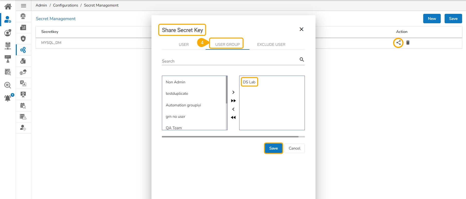
Share the configured Secret Management key to a user group.
Access a Data Science Notebook from a user account that is part of the User group with which the configured secret is shared.
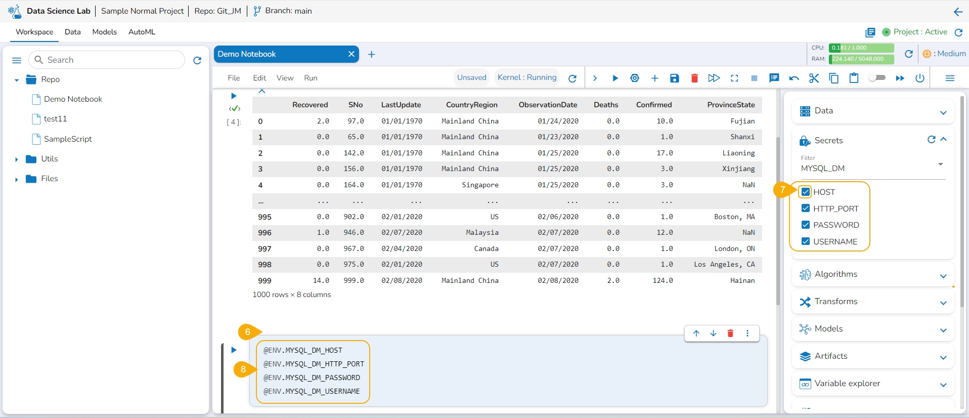
Open the Secrets tab from the right side.
Use the Refresh icon to get the latest configured Secret Key.
The newly created Secret Key is listed below. Click on a Secret Key option.
The selected Secret Key name option is displayed with a drop-down icon. Click the drop-down icon next to the Secret Key name to get the fields.
Add a new Code cell.
Select the Secret Keys by using the given checkboxes.
The encrypted environment variables for the fields are generated in the code cell.
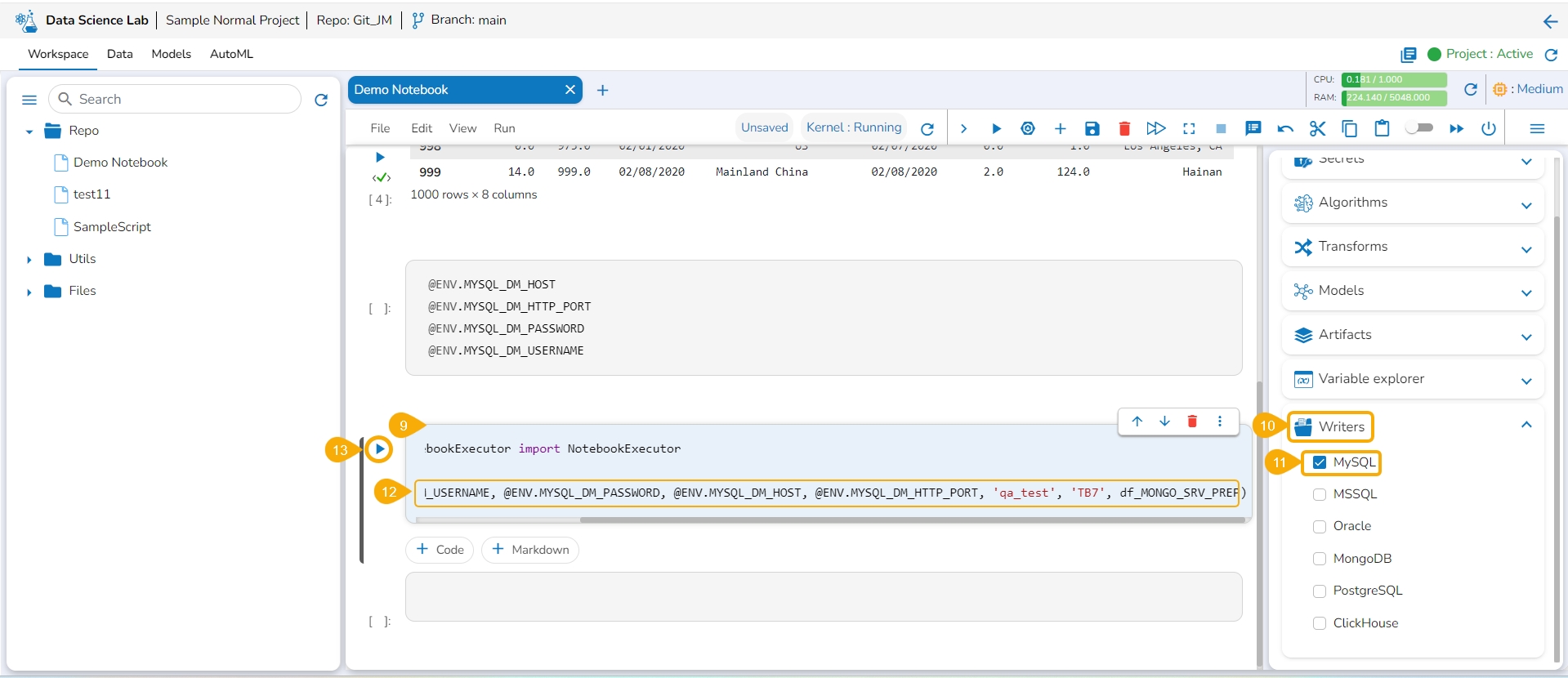
Add a new Code cell.
Open the Writers tab.
Select a writer type using the checkbox. E.g., In this case, MySQL has been selected.
Map the encrypted secret keys for the related configuration details like Username, Password, Port, Host, and Database by copying them.
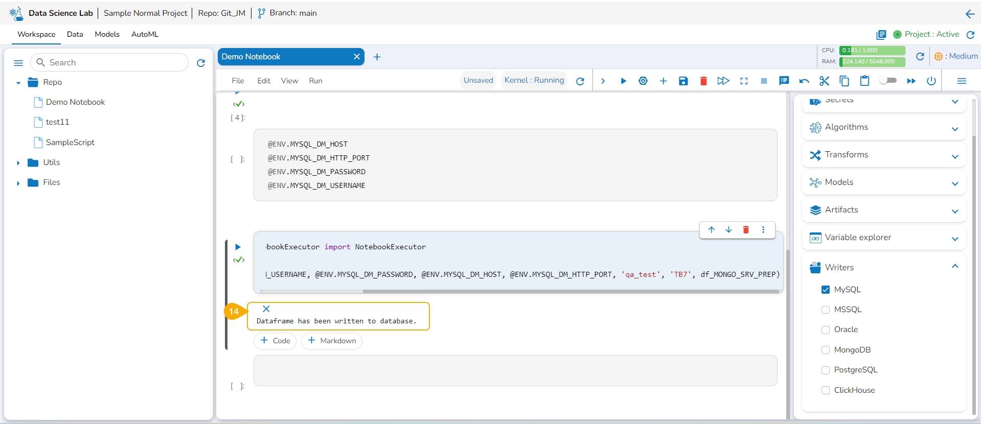
Run the cell.
The data frame will be written to the selected writer's database.
The Data options enables a user to add data inside their project from the Data Science Notebook infrastructure.
Navigate to a Data Science Notebook page (.ipynb file).
Click the Data icon given in the right side panel.
The Data option opens displaying the related icons.
Click on the Add icon.
The Add Data page appears.
The steps to add data may vary based on the selected Data source.
Please Note: Refer to the Adding Data page for more details on how to add data.
Please refer to these links: Adding Data Sets, Uploading and Adding Data Sandbox files, and Adding Feature Stores
Please Note: Using the get_data function datasets and data sandbox files (csv & xlsx files) can be read.
Add a new Code cell to Notebook or access an empty Code cell.
Select a dataset from the Data tab.
The get_data function appears in the code cell.
Provide the df (DataFrame) to print the data from the selected Dataset. A Dataset can be an added dataset, data sandbox file, or feature store.
Run the cell.
The Data preview appears below after the cell run is completed.
The Data Sets/ Sandbox files/ Feature Stores added to a Data Science Notebook will also be listed under the Data tab provided under the same project. Hence, the added datasets will be available for all the Data Science Notebooks created or imported under the same project.
Check out the illustration to read multiple sheets in a Notebook cell.
Add an Excel file with multiple sheets to a DS Project.
Insert a Markdown cell with the names of the Excel sheets.
Insert a new code cell.
Use a checkbox next to read data.
The get_data function in the code cell.
Run the code cell.
The data preview will appear below.
Select another datasheet name and copy it from the markdown cell.
Paste the copied datasheet name in the code cell that contains the get_data function.
Run the code cell.
The data preview will be displayed below.
Get steps on how to do Algorithm Settings and Project level access to use Algorithms inside Notebook.
Pre-requisite:
Configure the Algorithms using the Data Science Lab Settings from the Admin module to access them under the Data Science Lab Project creation.
The user must select Algorithms while creating a Project to make them accessible for a Notebook within the Project.
The entire process to access the Algorithms option inside the DS Lab and actually create a model based on the Algorithm is a three-step process:
Please Note: The first two steps are prerequisites for the user to avail desired Algorithms inside their DS Lab Projects.
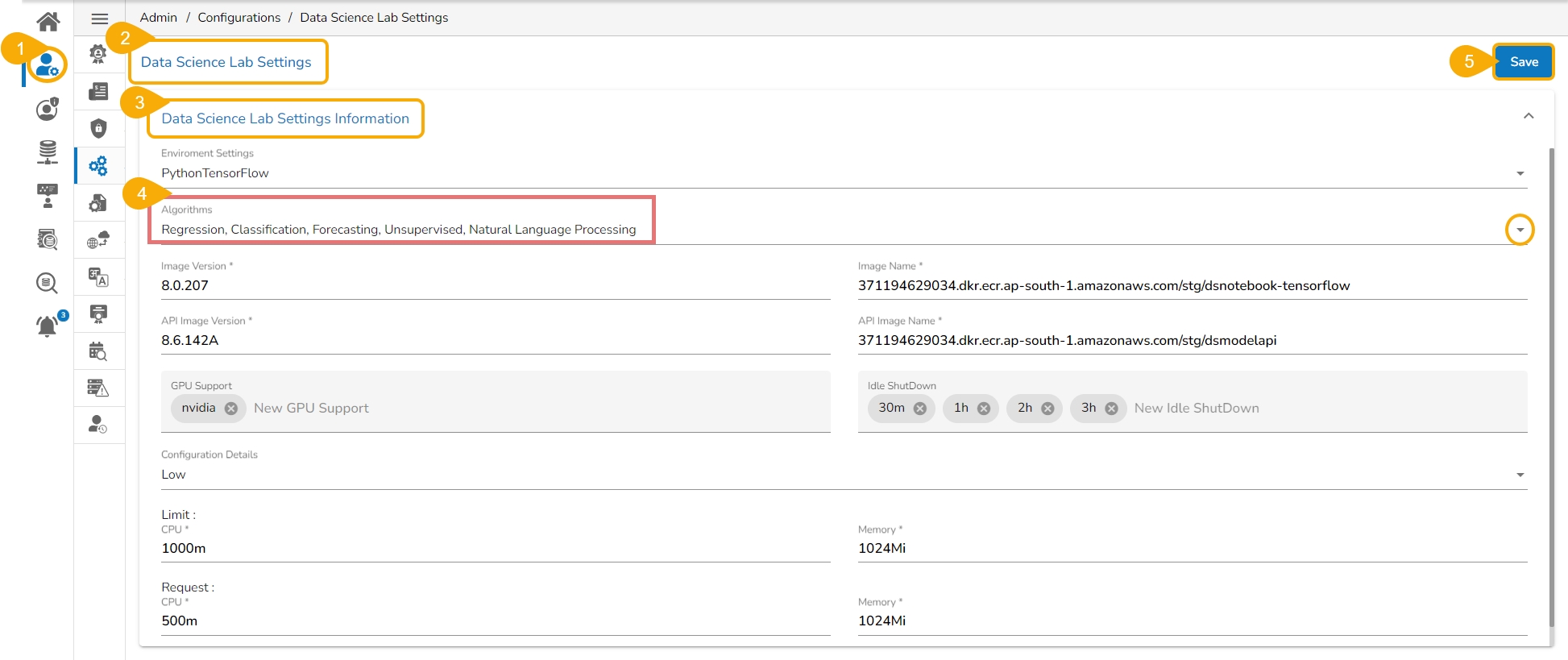
Navigate to the Admin module.
Open the Data Science Settings option from the Configuration section of the Admin panel.
The Data Science Settings Information page opens.
Select the Algorithms using the drop-down option.
Click the Save option.
A confirmation message appears to inform about the Notebook details updates.
Please Note:
Regression & Classification - Default Algorithm types that Admin will enable for each Data Science Lab module user.
Forecasting, Unsupervised, Natural Language Processing - These algorithms will be disabled by default. As per the user's request, they will be enabled by the Admin.
Once the Algorithm settings are configured in the Admin module, and the required Algorithms are selected while creating a Data Science Project, the user can access those Algorithms within a Notebook created under the same DSL Project.
Please Note: Once the Algorithm configuration is completed from the Admin and Project level the same set of Algorithms will be available for all the Notebooks which are part of that DSL Project.
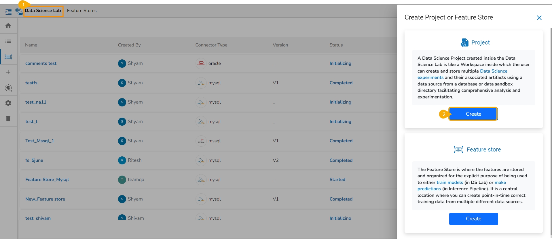
Navigate to the Data Science Lab.
Click the Create option for Project.
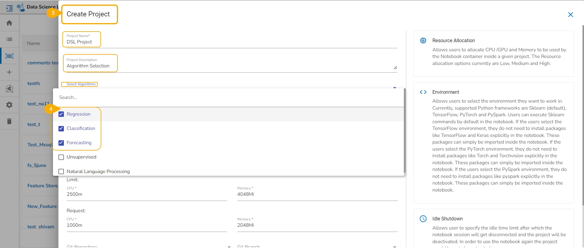
The Create Project page appears.
Select the algorithms using the given checkboxes from the drop-down menu.
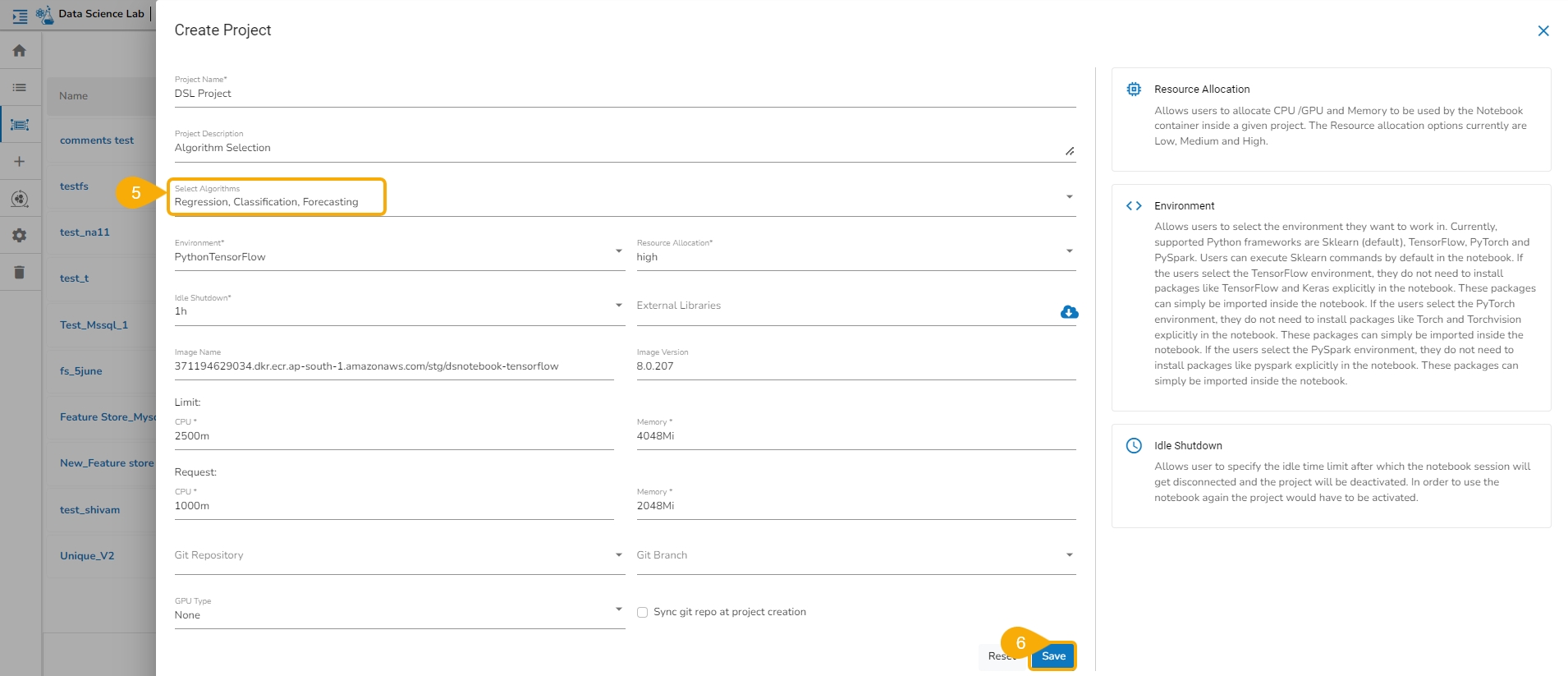
The selected Algorithms appear on the field separated by a comma.
Save the project.
Please Note: Provide all the required fields for the Project creation.
Once the Algorithms are selected while creating a Project, those algorithms will be available for all the Notebooks created inside that project.
Prerequisite:
Please activate the Project to access the Notebook functionality inside it.
Do the required Admin level Settings and Project Level settings to access the Algorithms inside a Data Science Lab Notebook.
Check out the illustration on using an algorithm script inside a Data Science Notebook.
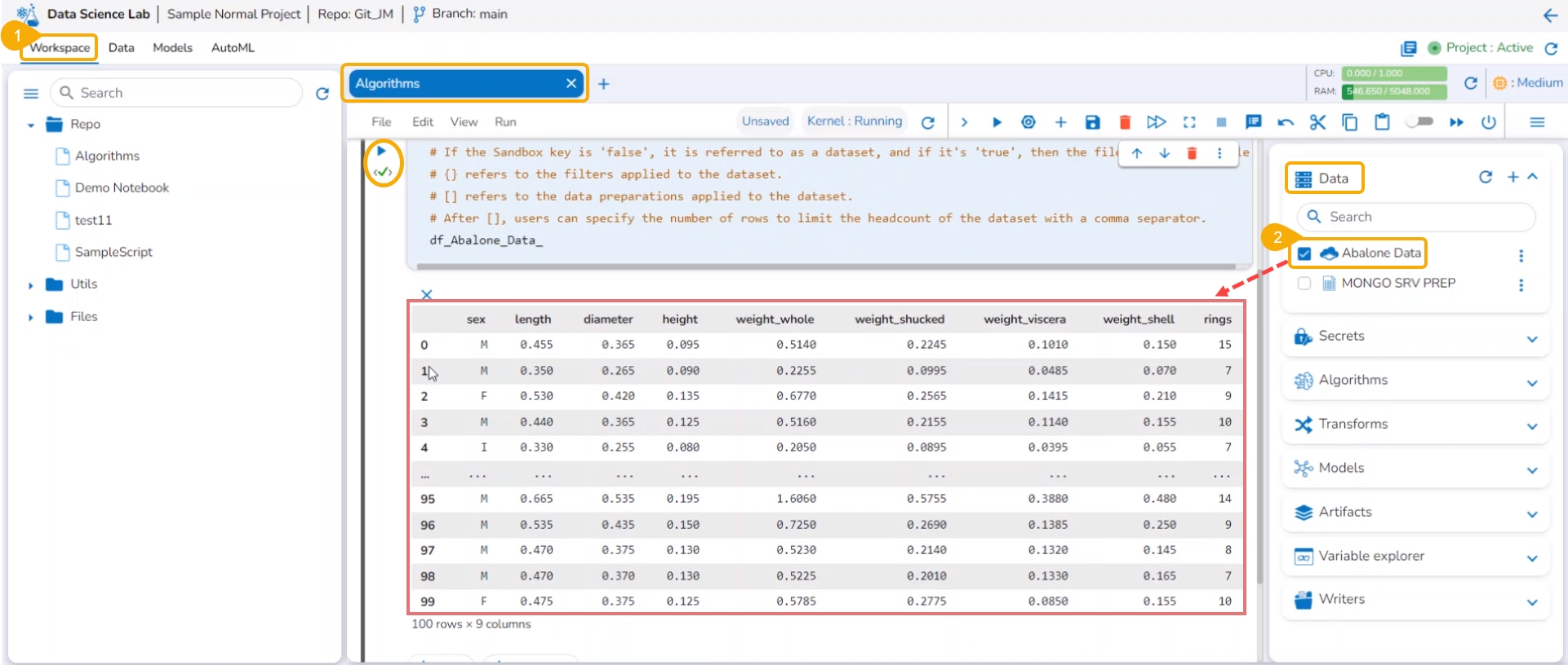
Navigate to the Workspace tab inside the same Project.
Add a dataset and run it.
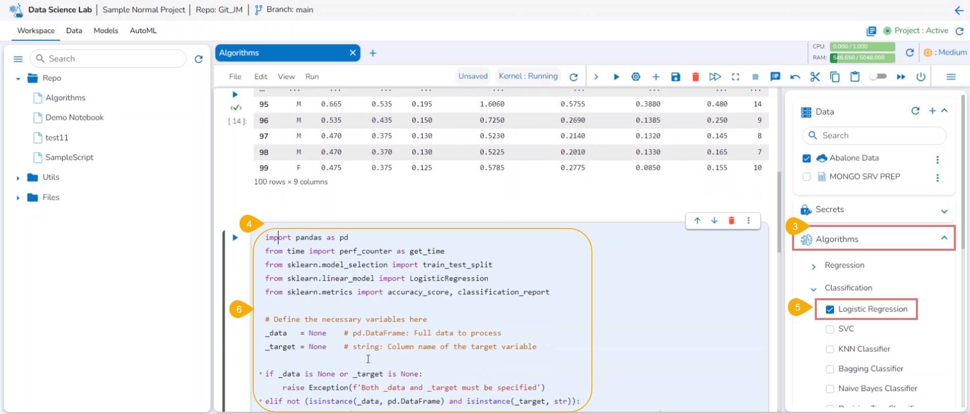
Click the Algorithms tab.
Add a new code cell in the .ipynb file.
It will display the list of algorithms selected and added at the Project level. Select a sub-category of the Algorithm using a checkbox.
The pre-defined code for the selected algorithm type gets added to the code cell.
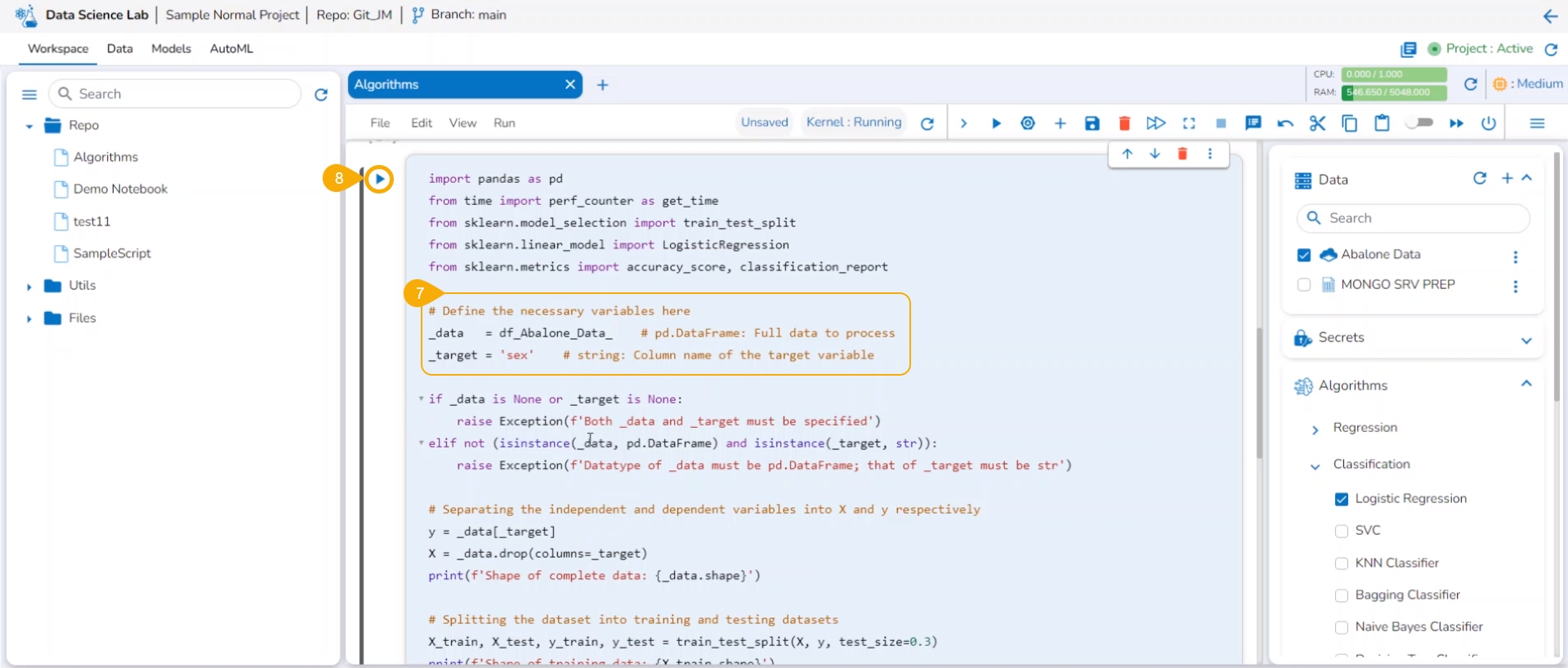
Define the necessary variables in the code cell. Define the Data and Target column in the auto-generated algorithm code.
Run the code cell.
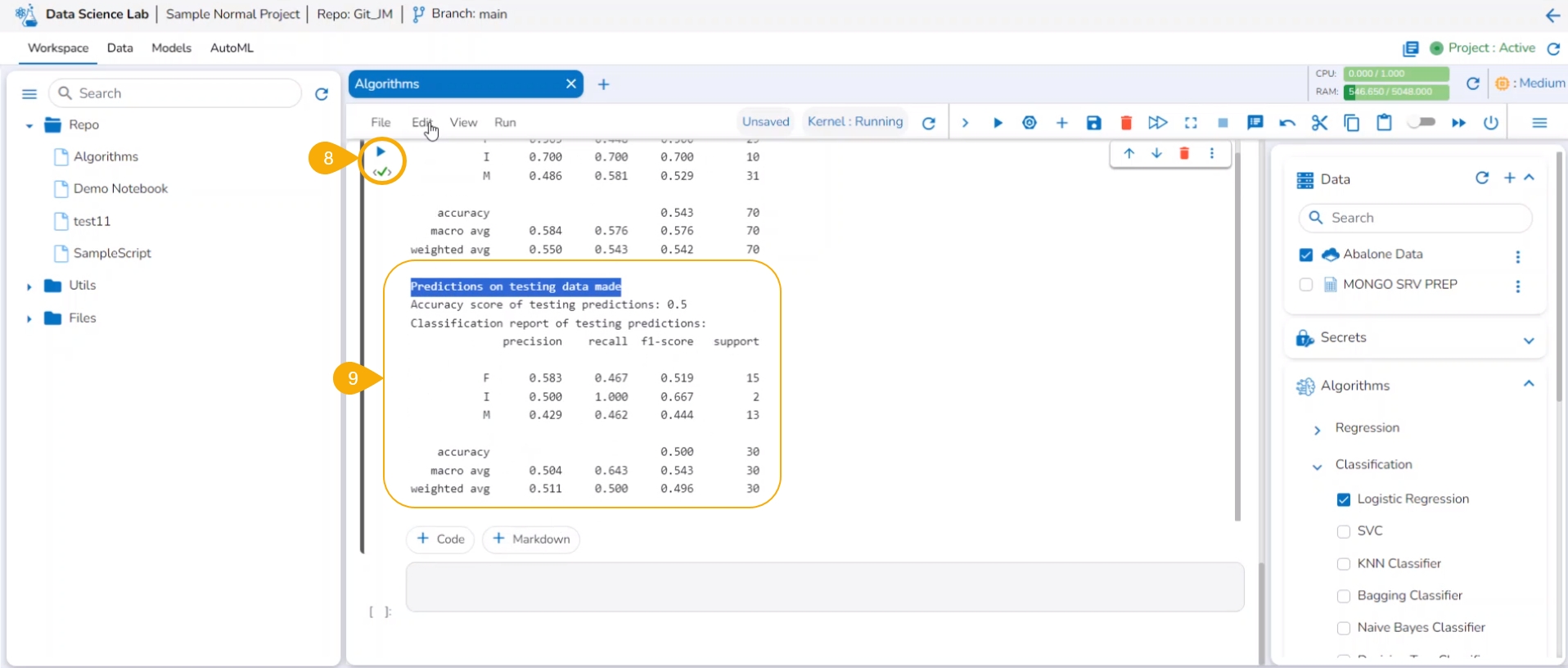
After the code cell run is completed.
The test data predictions based on the train data appear below.
Please Note:
To see the output, you can run the cell containing the data frame details.
The model based on the Algorithm can be saved under the Models tab.
The algorithm-based models can be registered to be accessed inside the Data Pipeline module.
The model based on an Algorithm script can be registered as an API service. Refer to the Register a Model as an API Service section for more details.
The Algorithm section within the Workspace offers a wide array of powerful out-of-the-box solutions across five key categories:
Please Note: Access to the sub-categories Forecasting, Unsupervised Learning, and Natural Language Processing requires administrator enablement. By default, all users can view and access Regression and Classification algorithms.
This section aims at describing the various operations for a Data Science Notebook.
Please Note: The Notebook Operations may differ based on the selection of the project environments. A notebook created under the PySpark environment only supports Data, Secrets, Variable Explorer, and Writers operations.
A Data Science Notebook created under the PyTorch or TensorFlow environment will contain the following operations:
Data: Add data and get a list of all the added datasets.
Secrets: You can generate Environment Variables to save your confidential information from getting exposed.
Algorithms: You can get steps to do Algorithm Settings and Project-level access to use Algorithms inside Notebook.
Transforms: Save and load models with transform script, register them, or publish them as an API through the DS Lab module.
Models: You can train, save, and load the models (Sklearn, Keras/TensorFlow, PyTorch). You can also register a model using this tab. Refer to Model Creation using Data Science Notebook for more details.
Artifacts: You can save the plots and datasets as Artifacts inside a DS Notebook.
Variable Explorer: Get detailed information on Variables declared inside a Notebook.
Writers: Write the DSL experiments' output into the database writers' supported range.
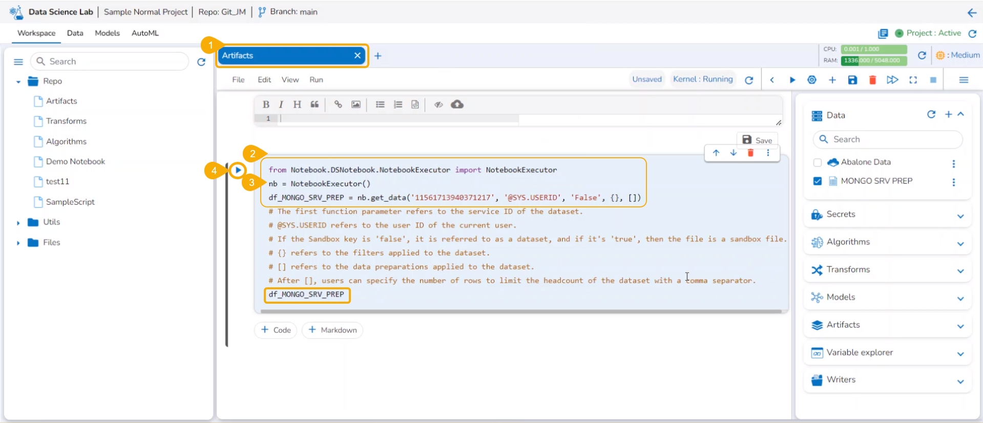
This section explains the steps to read the added Data inside a Data Science Notebook.
Please Note: Using the get_data function datasets and data sandbox files (csv & xlsx files) can be read.
Add a new Code cell to Notebook or access an empty Code cell.
Select a dataset from the Data tab.
The get_data function appears in the code cell.
Provide the df (DataFrame) to print the data from the selected Dataset. A Dataset can be an added dataset, data sandbox file, or feature store.
Run the cell.
The Data preview appears below after the cell run is completed.
The Data Sets/ Sandbox files/ Feature Stores added to a Data Science Notebook will also be listed under the Data tab provided under the same project. Hence, the added datasets will be available for all the Data Science Notebooks created or imported under the same project.
Check out the illustration to read multiple sheets in a Notebook cell.
Add an Excel file with multiple sheets to a DS Project.
Insert a Markdown cell with the names of the Excel sheets.
Insert a new code cell.
Use a checkbox next to read data.
The get_data function in the code cell.
Run the code cell.
The data preview will appear below.
Select another datasheet name and copy it from the markdown cell.
Paste the copied datasheet name in the code cell that contains the get_data function.
Run the code cell.
The data preview will be displayed below.
Get the Variables information listed under this tab.
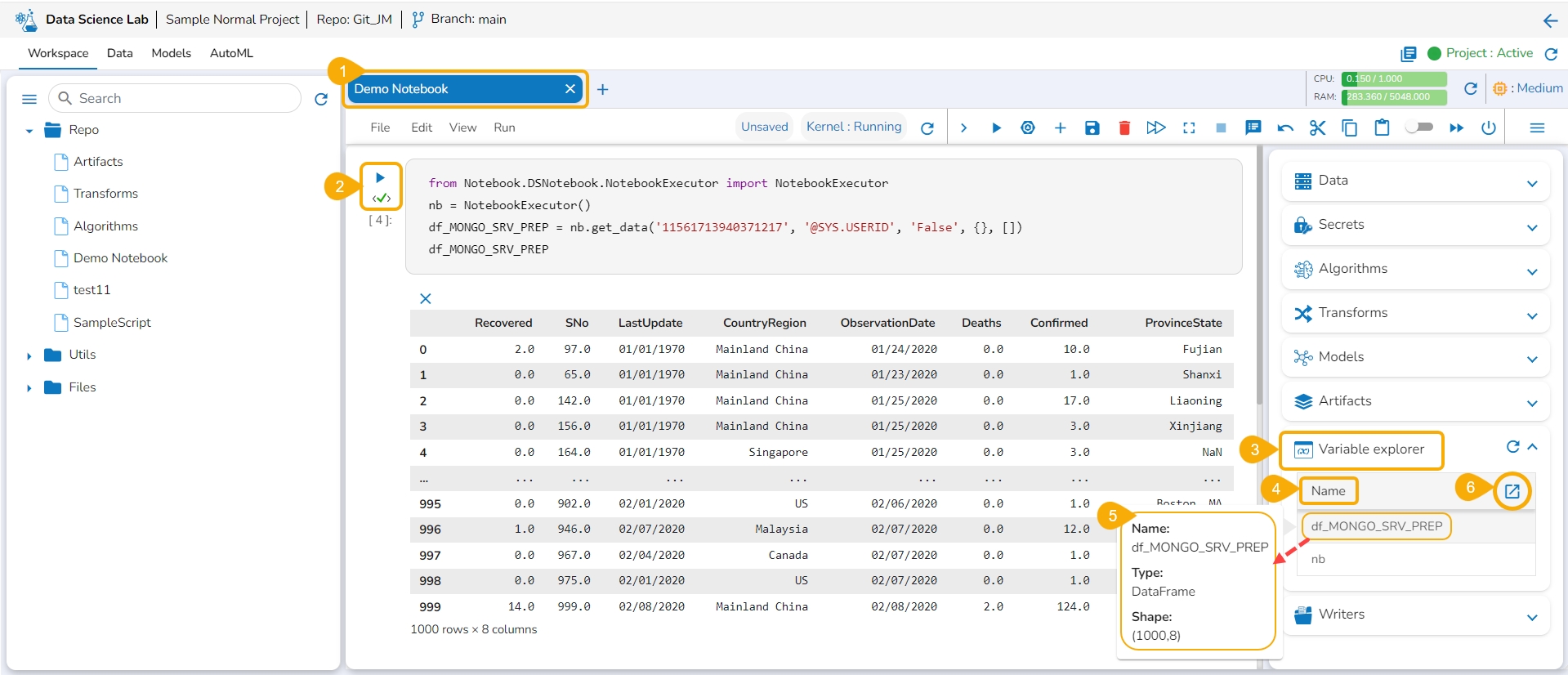
The Variable Explorer tab displays the Name column and Explore icon for all the variables created and executed within the Notebook cells.
Navigate to the Notebook page.
Write and run code using the Code cells.
Open the Variable Explorer tab.
The variables will be listed below under the Name column.
By hovering the cursor on a variable, you can get a mention of the name, type, and shape details of the selected variable.
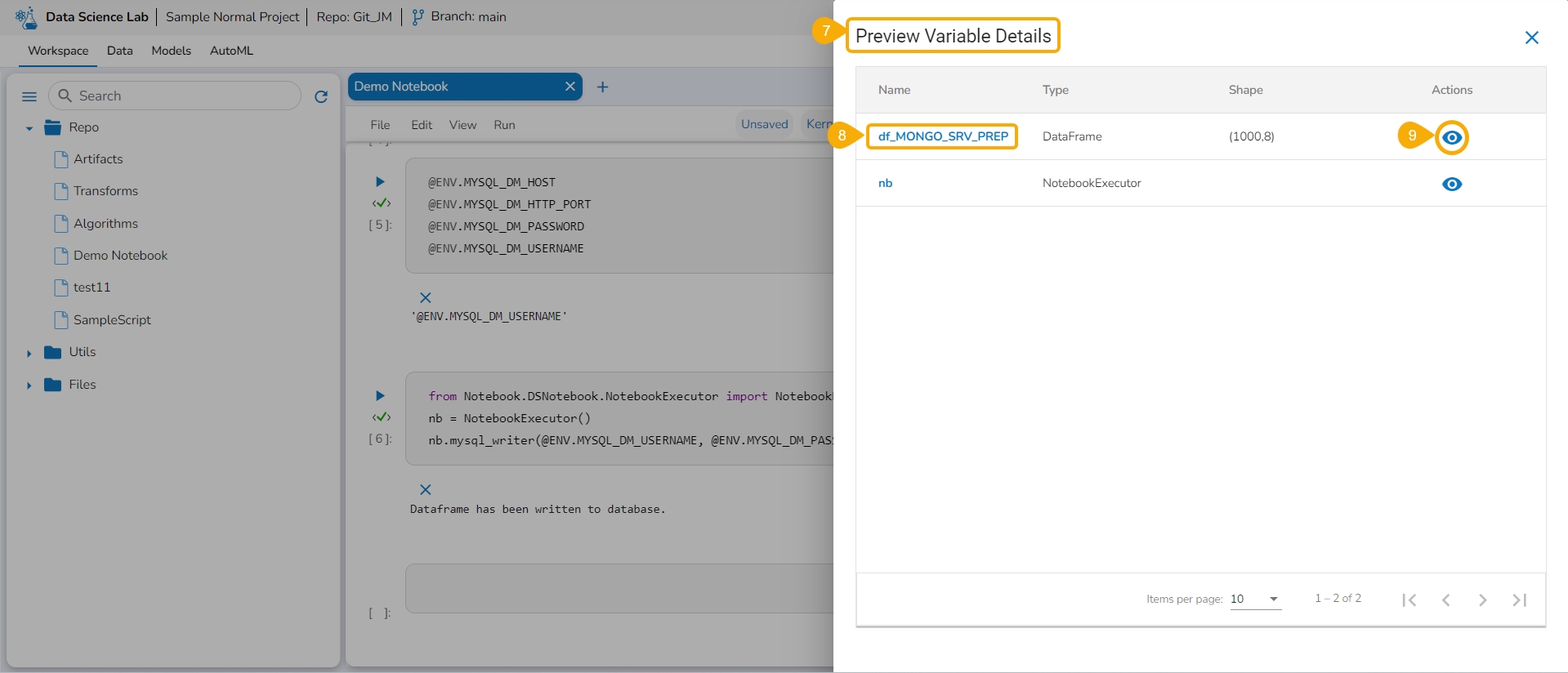
Click the Explore icon.
The Preview Variable Details page opens.
Select a Variable from the displayed list.
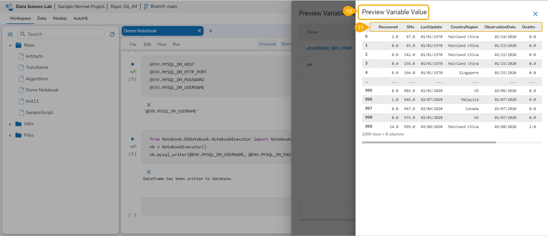
Click the Preview icon provided for the selected Variable.
The Preview Variable Value page opens.
All the values of the selected Variable are displayed in a tabular format.
This page explains how to save Artifacts. Users can save plots and datasets inside a DS Notebook as Artifacts.
Check out the walk-through on how to Save Artifacts.
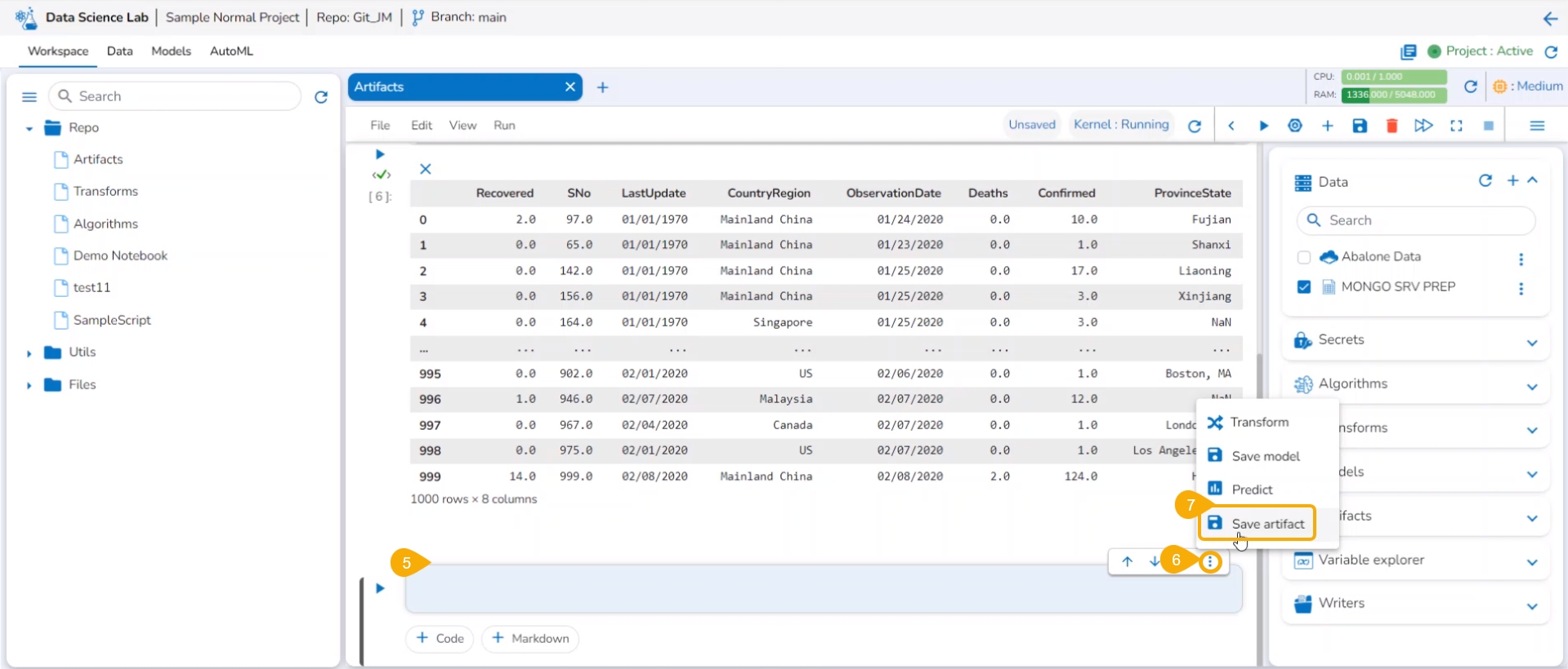
Navigate to a Data Science Notebook.
Add a new cell.
Provide Data set.
Define DataFrame and execute the cell.
A new cell will be added below.
Click the Ellipsis icon to access more options.
Select the Save Artifacts option.
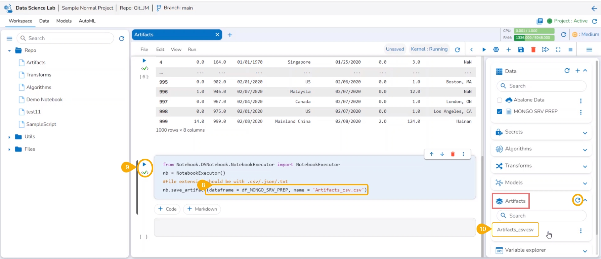
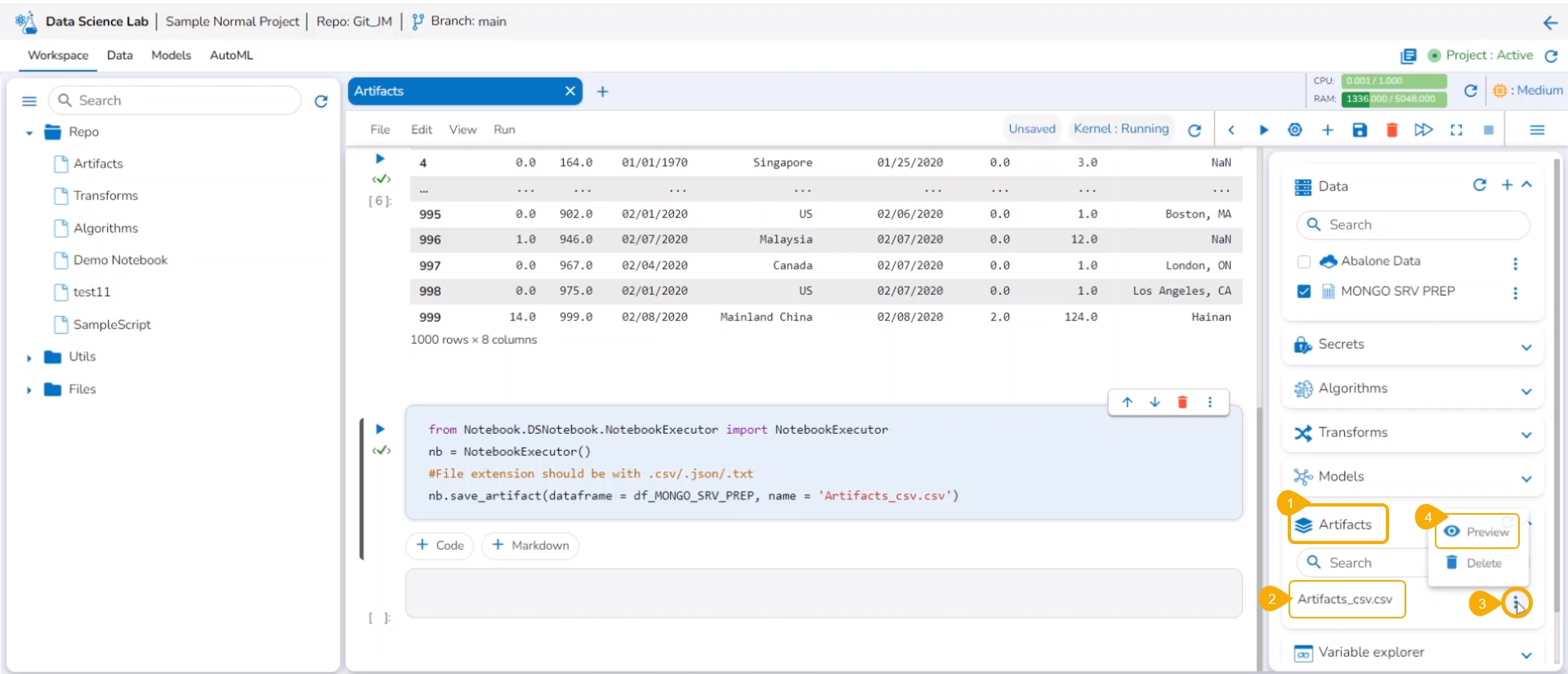
Give proper DataFrame name and Name of Artifacts (with extensions - .csv/.txt/.json)
Execute the cell.
The Artifacts get saved under the Artifacts tab.
Please Note:
The saved Artifacts can be downloaded as well.
The user can also get an instant visual depiction of the data based on their executed scripts.
Navigate to the Artifacts tab inside a DS Notebook page.
Select a saved Artifact from the right side panel.
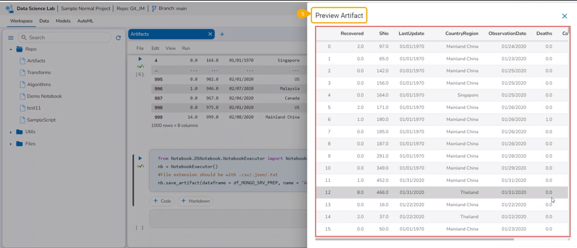
Click the Preview option from the context menu.
The Artifact Preview gets displayed.
Please Note:
The selected Artifact gets deleted from the list by clicking the Delete option.
Save and load models with transform script, register them or publish them as an API through DS Lab module.
Check out a walk-through on how to use the Transform script inside Notebook.
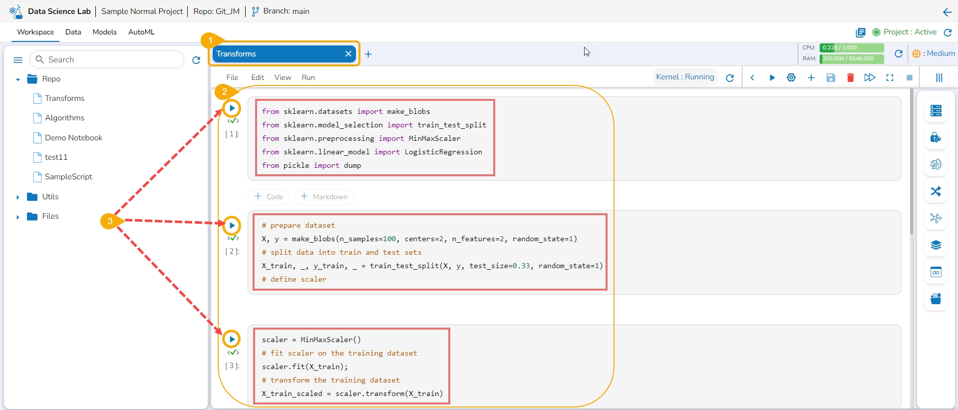
You can write or upload a script containing the transform function to a Notebook and save a model based on it. You can also register the model as an API service. This entire process is completed in the below-given steps:
Navigate to a Notebook.
Add a Code cell. Write or provide a transform script to the cell (In this case, it has been supplied in three cells).
Run the cell(s) (In this case, run all the three cells).
Add a new code cell and define the model.
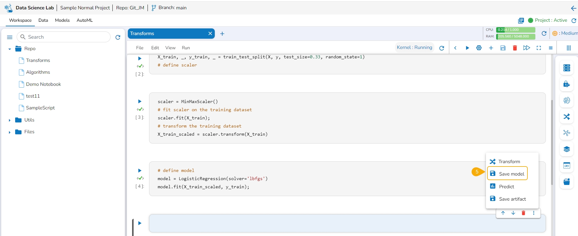
Add another cell and click the Save Model option for the newly added code cell.
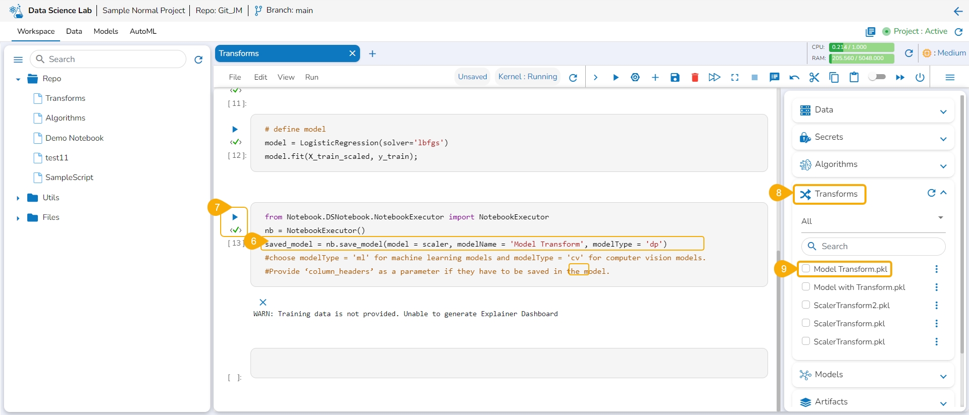
Specify the model name and type in the auto-generated script in the next code cell.
Run the cell.
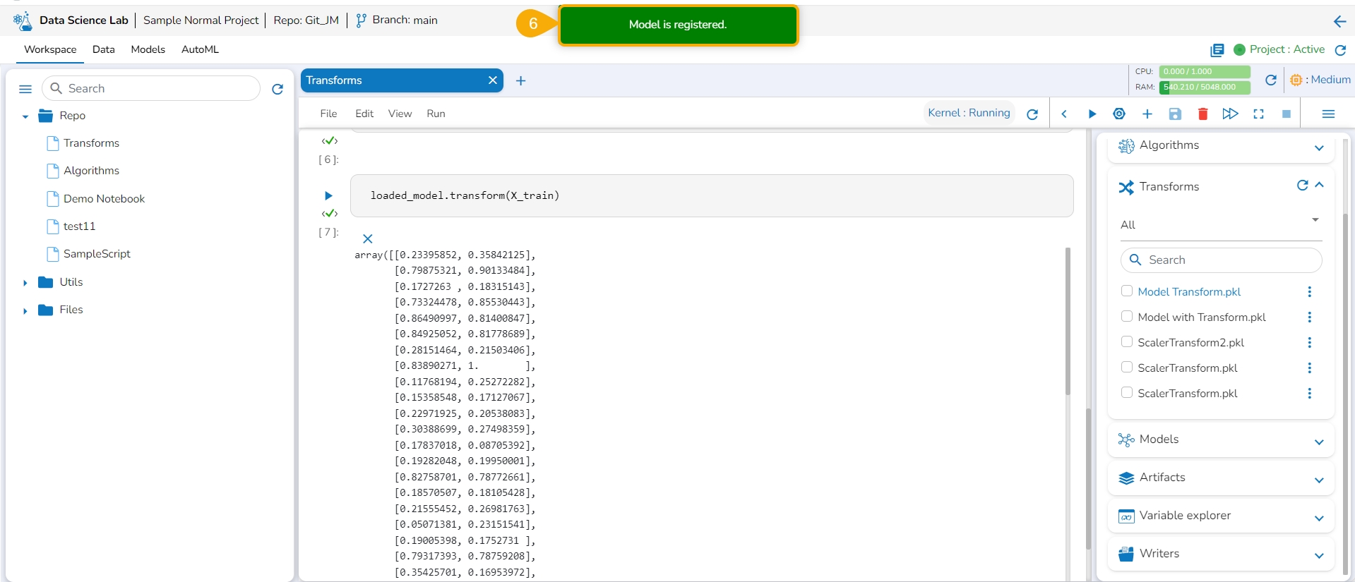
Open the Transforms tab.
The model gets saved under the Transforms tab.
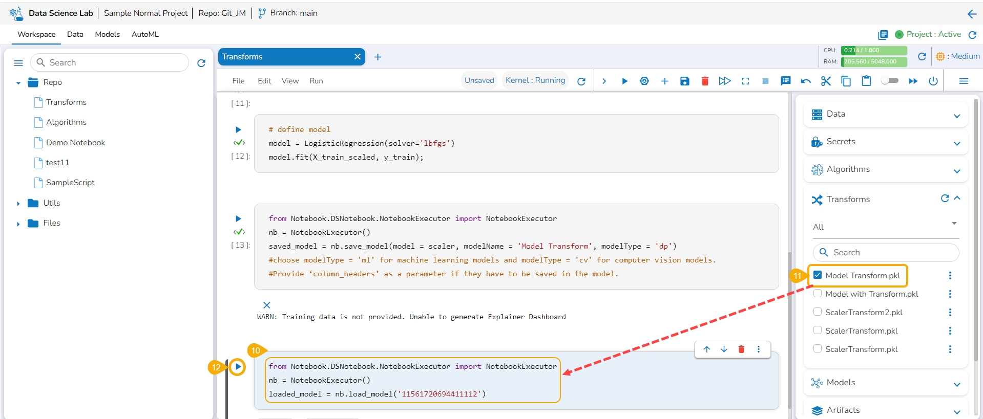
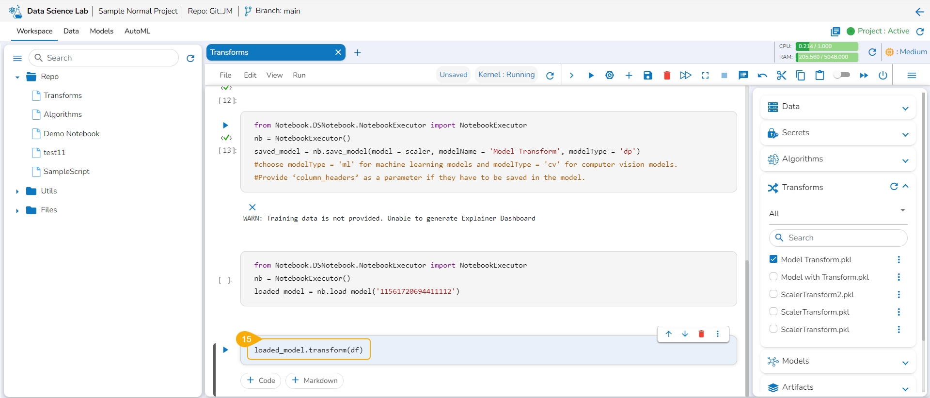
Add a new code cell.
Load the transform model by using the checkbox.
Run that cell.
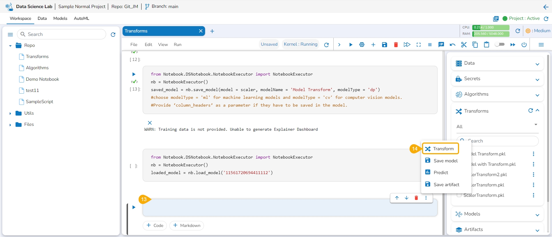
Insert a new code cell.
Click the Transforms option for the code cell.
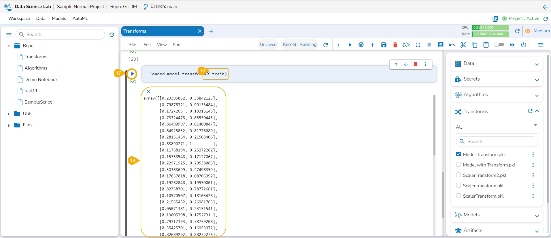
The auto-generated script appears.
Specify the train data.
Run the code cell.
It will display the transformed data below.
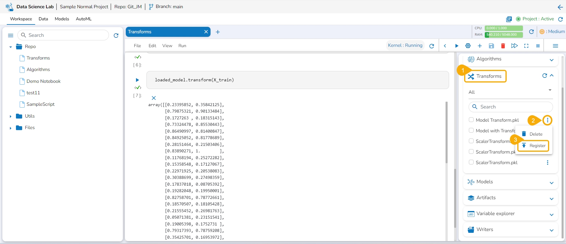
Open the Transforms tab inside a Notebook.
Click the ellipsis icon for the saved transform.
Select the Register option for a listed transform.
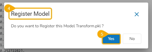
The Register Model dialog box opens to confirm the action.
Click the Yes option.
A confirmation message appears to inform the completion of the action.
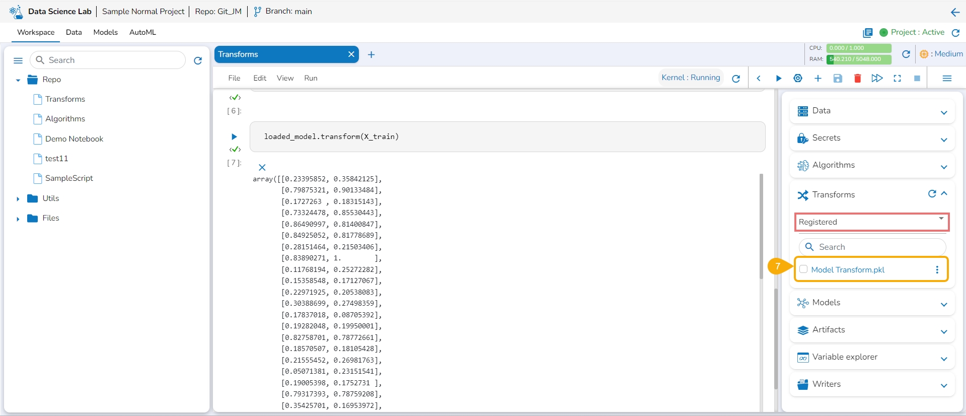
The model gets registered and listed under the Registered list of the models.
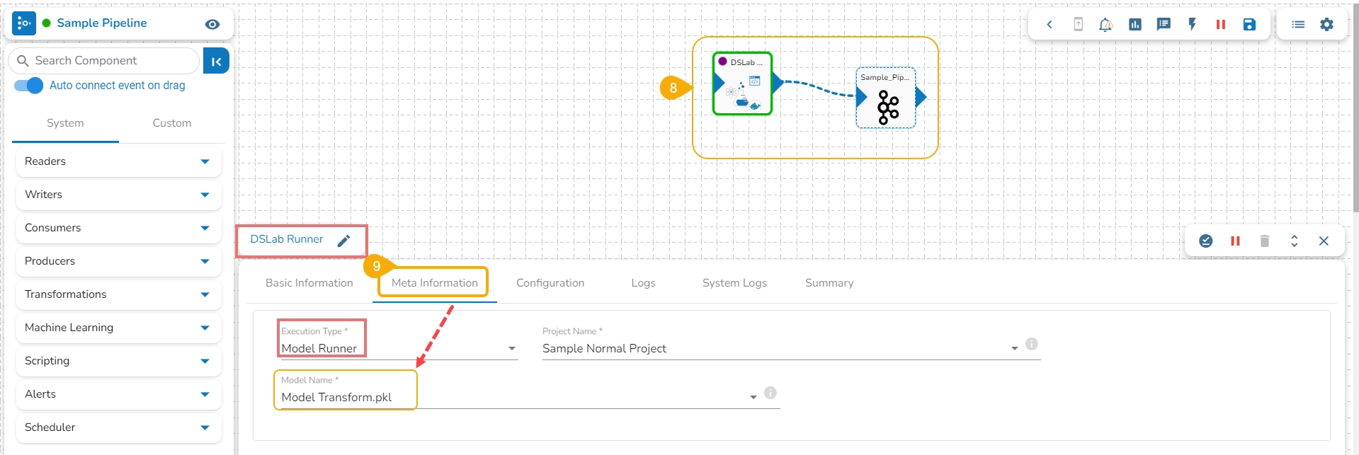
Open a pipeline workflow with a DS Lab model runner component.
The registered model gets listed under the Meta Information tab of the DS Lab model runner component inside the Data Pipeline module.
The steps to publish a model as an API that contains transform remain the same as described for a Data Science Model. Refer to the Register a Model as an API Service page.
This page explains the Writers tab available in the right-side panel of the Data Science Notebook.
The Data Science Lab module provides a Writers tab inside the Notebook to write the output of the data science experiments.
Check out the illustration on how to use the Writers operation inside a DS Notebook.
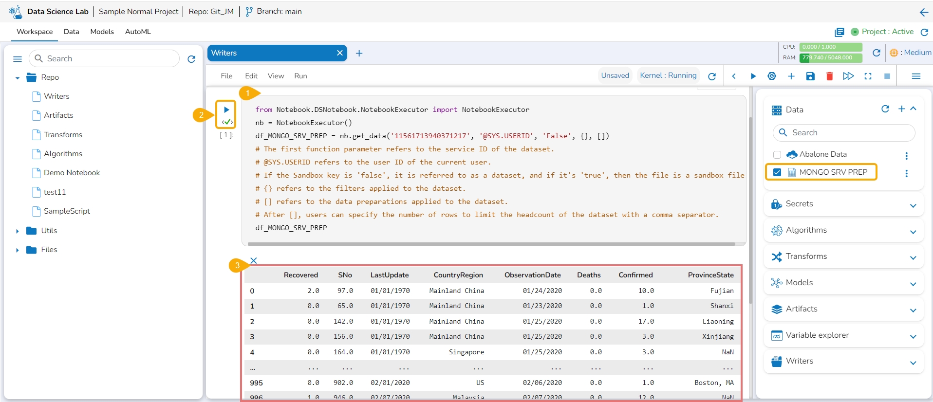
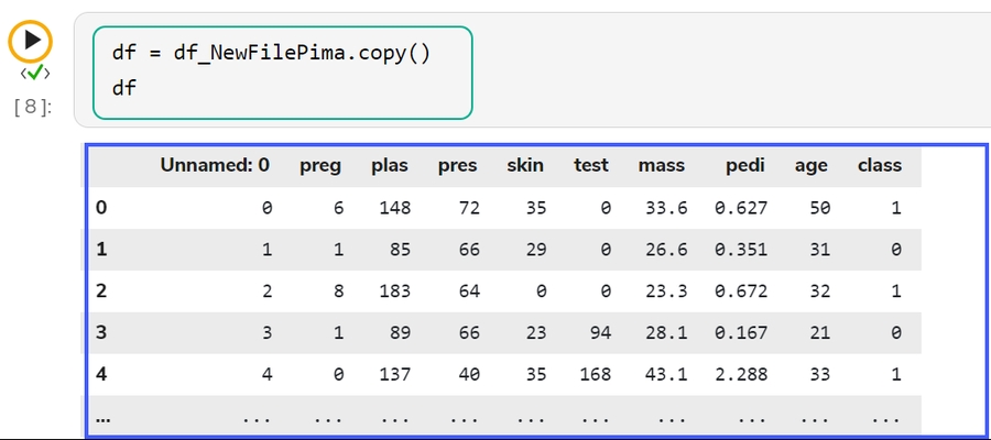
Navigate to a code cell with dataset details.
Run the cell.
The preview of the dataset appears below.
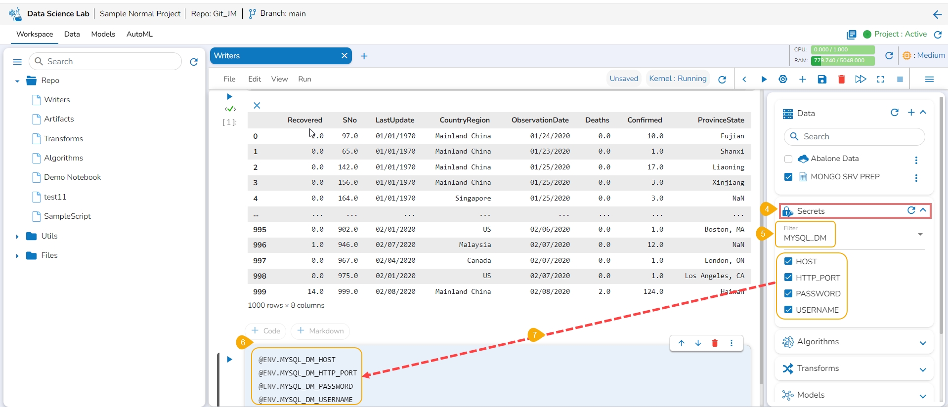
Click the Secrets tab to get the registered DB secrets.
Select the registered DB secret keys from the Secrets tab.
Add a new code cell.
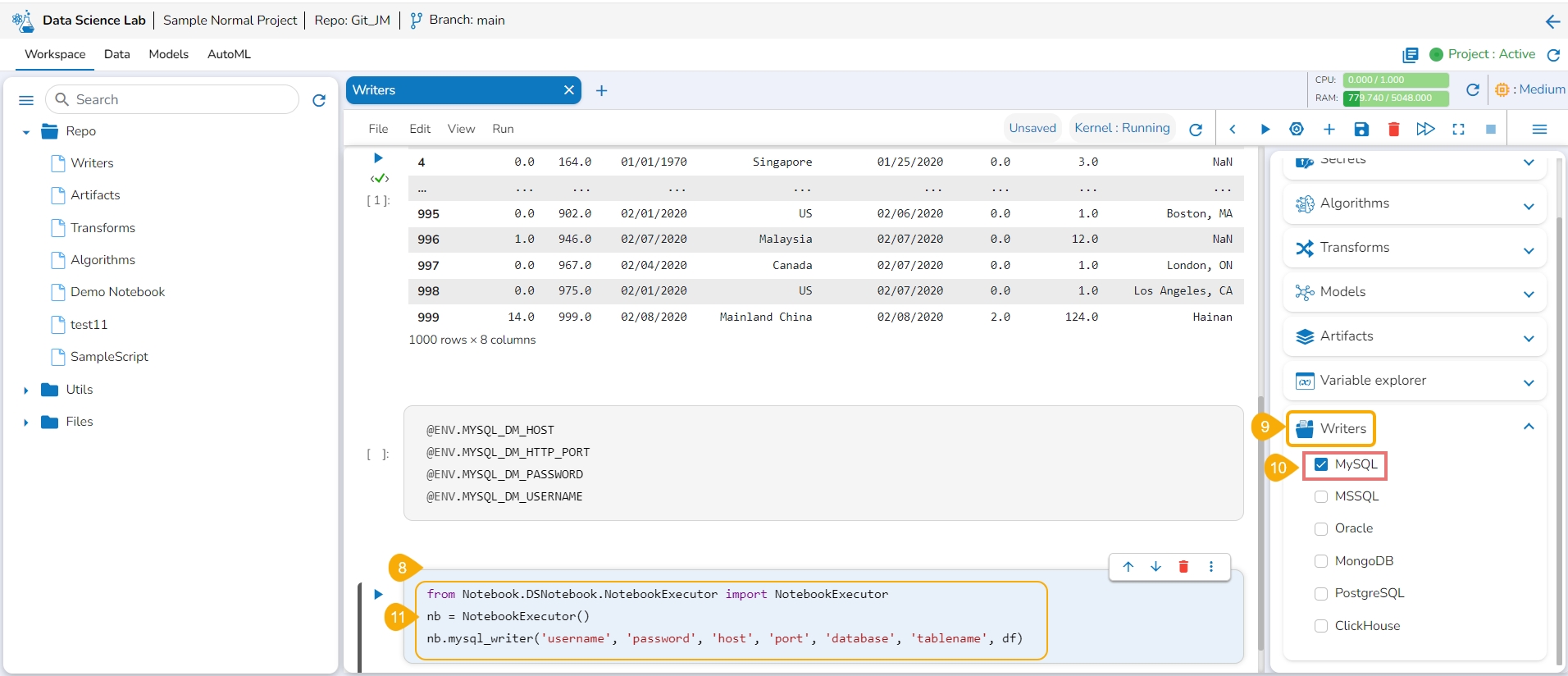
Get the Secret keys of the DB using the checkboxes provided for the listed Secret keys.
Add a new code cell.
Open the Writers section.
Use the given checkbox to select a driver type for the writers.
The code gets added to the newly added cell.
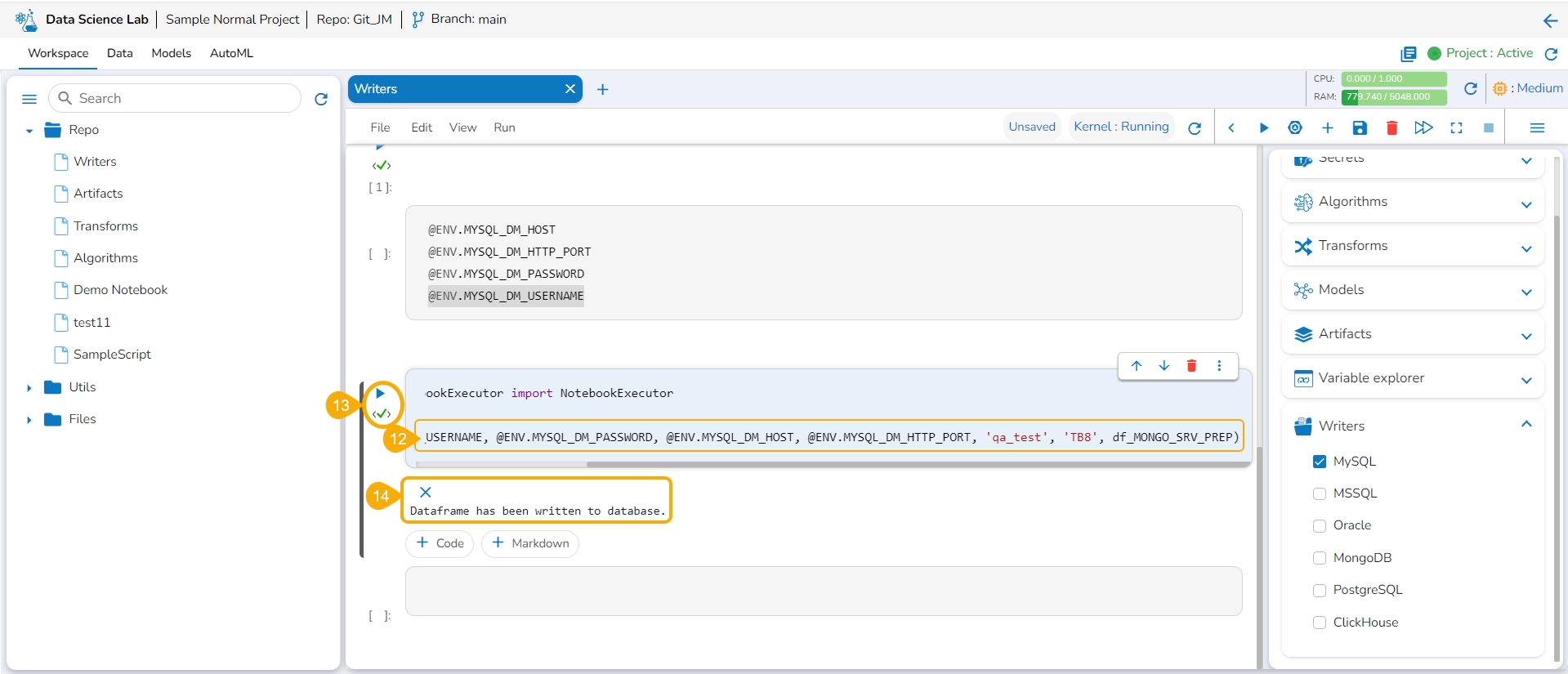
Provide the Secret values for the required information of the writer such as Username, Password, Host, Port, Database name, table name, and DataFrame.
Run the code cell with the modified database details.
A message below states that the DataFrame has been written to the database. The data gets written to the specified database.
Please Note: The supported DB writers are MYSQL, MSSQL, Oracle, MongoDB, PostgreSQL, and ClickHouse.
Click the vertical ellipsis icon for the saved Artifact.


