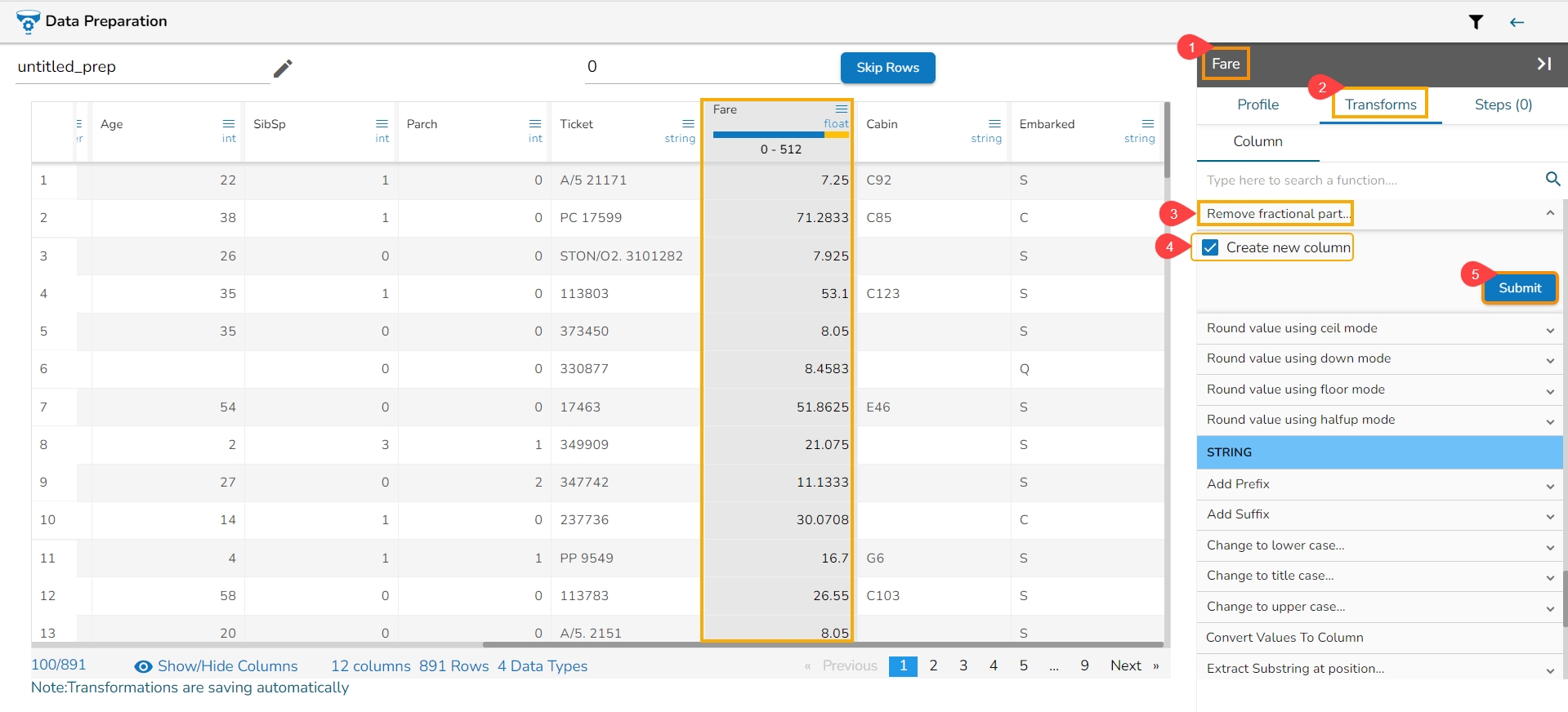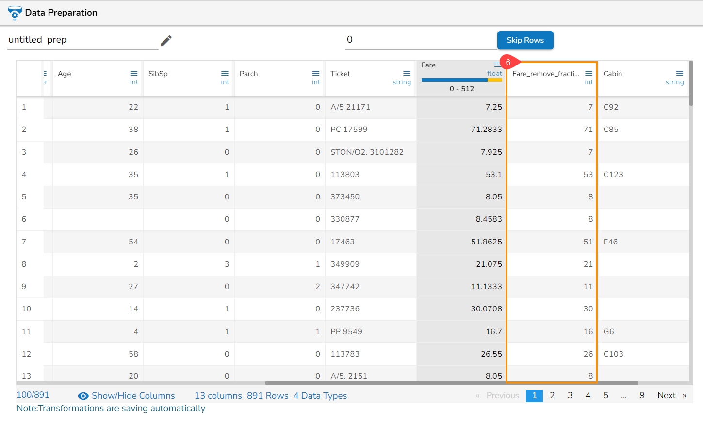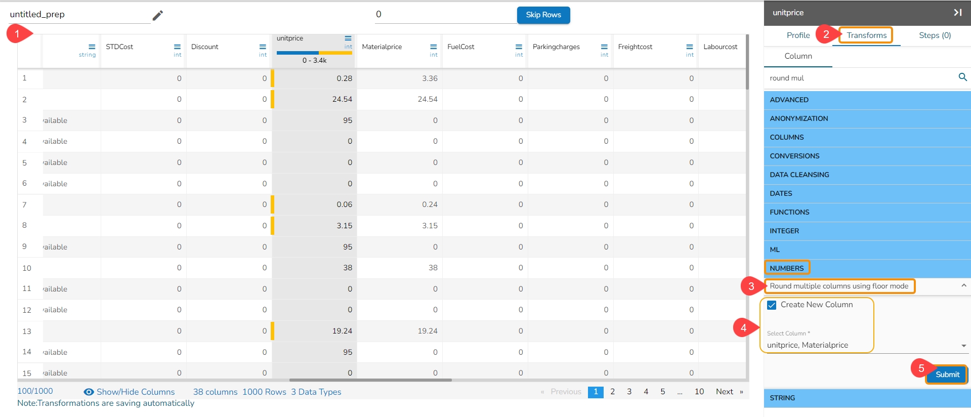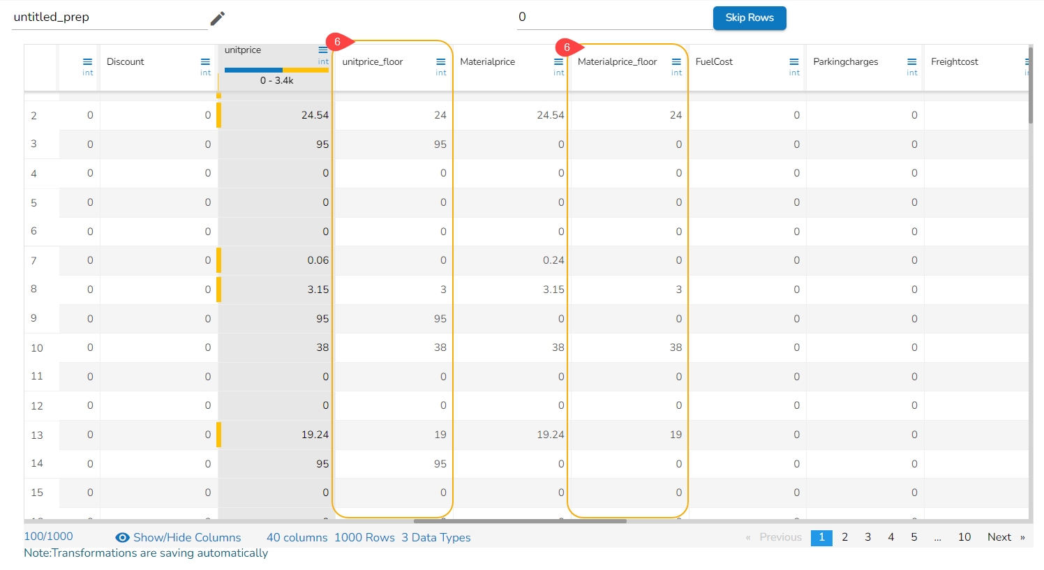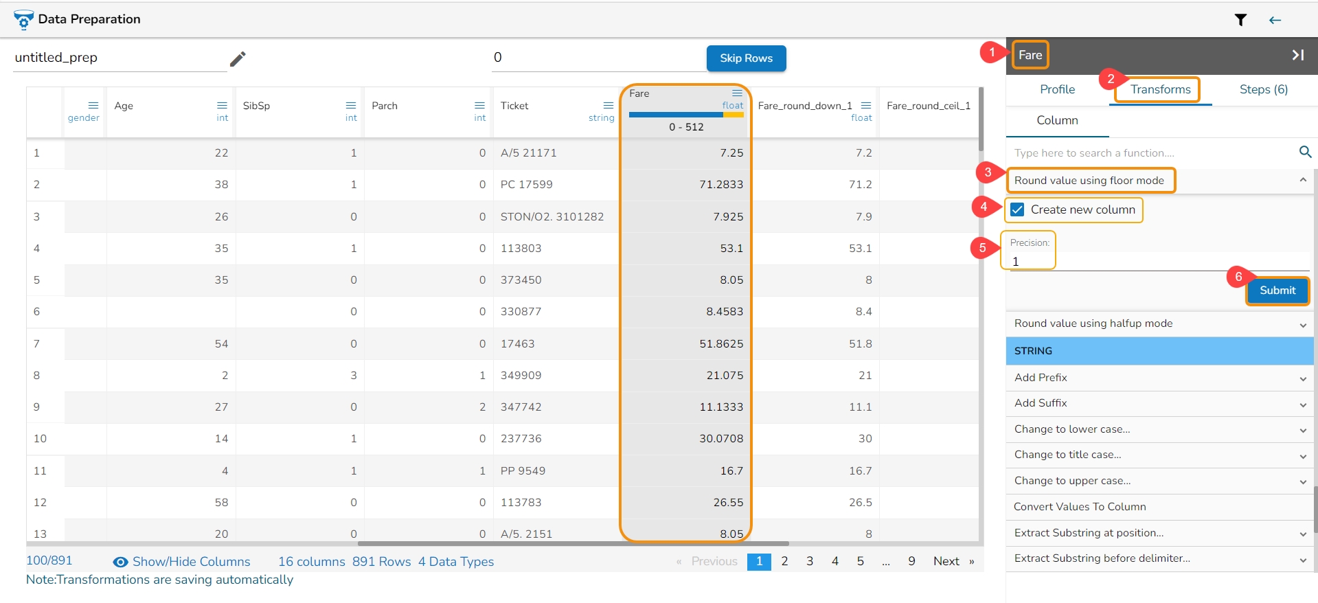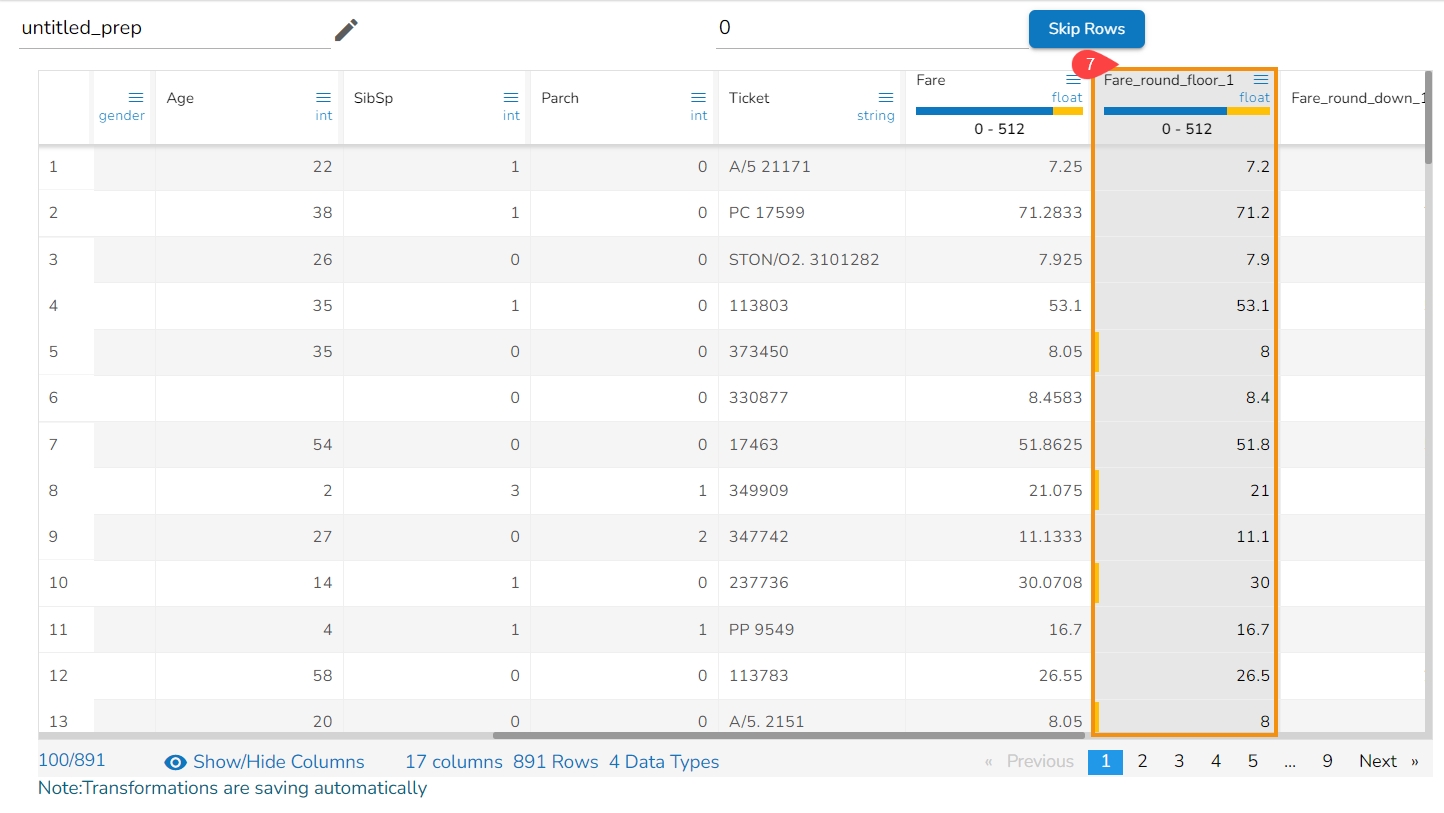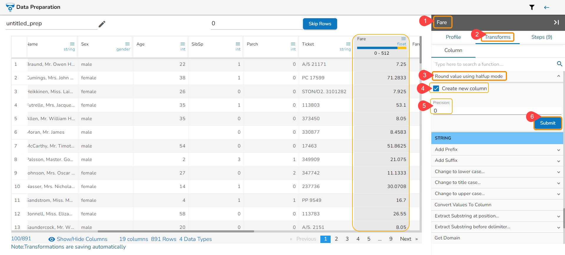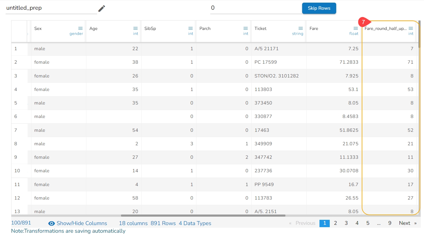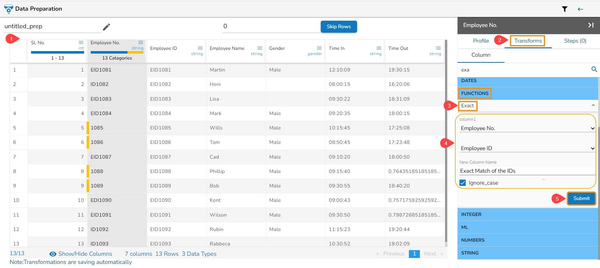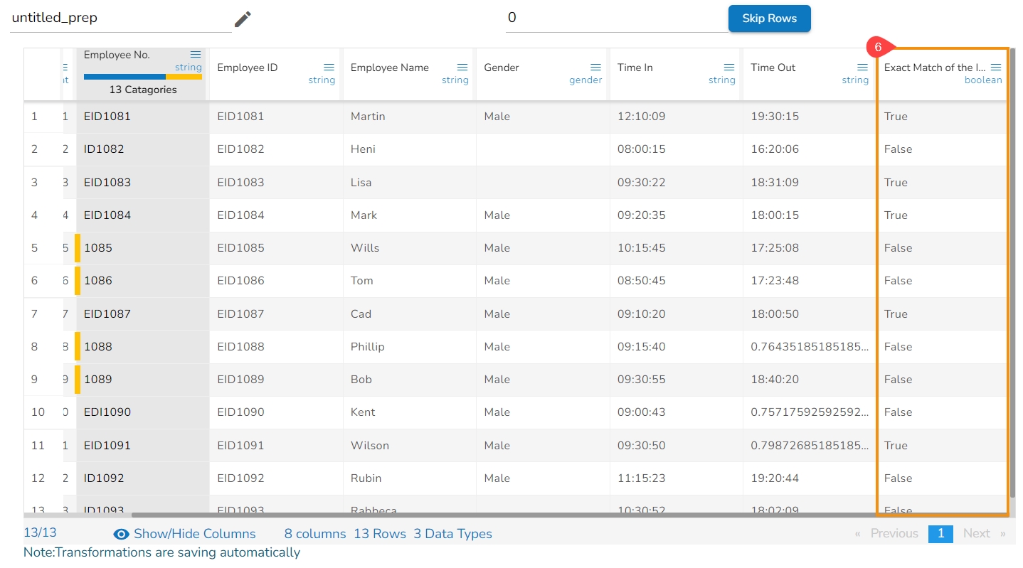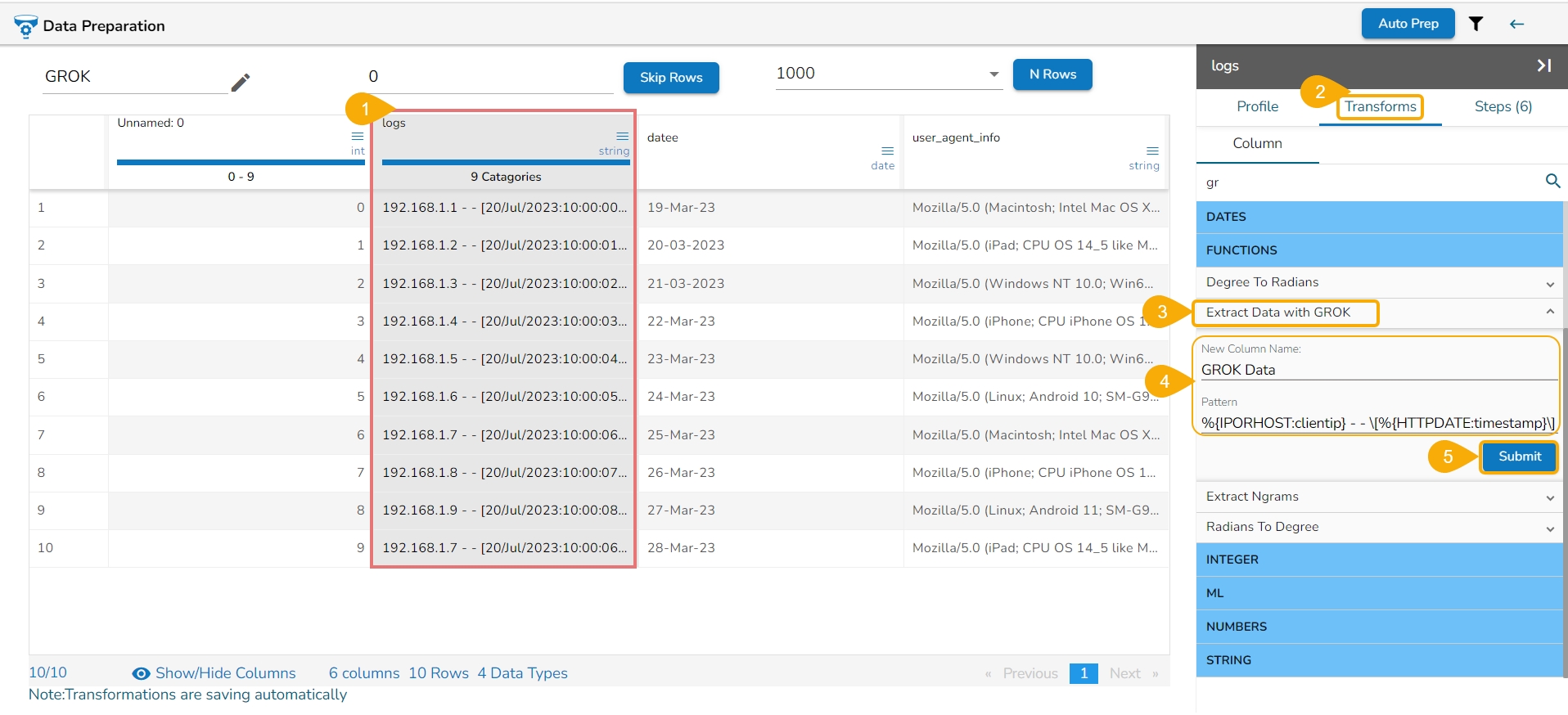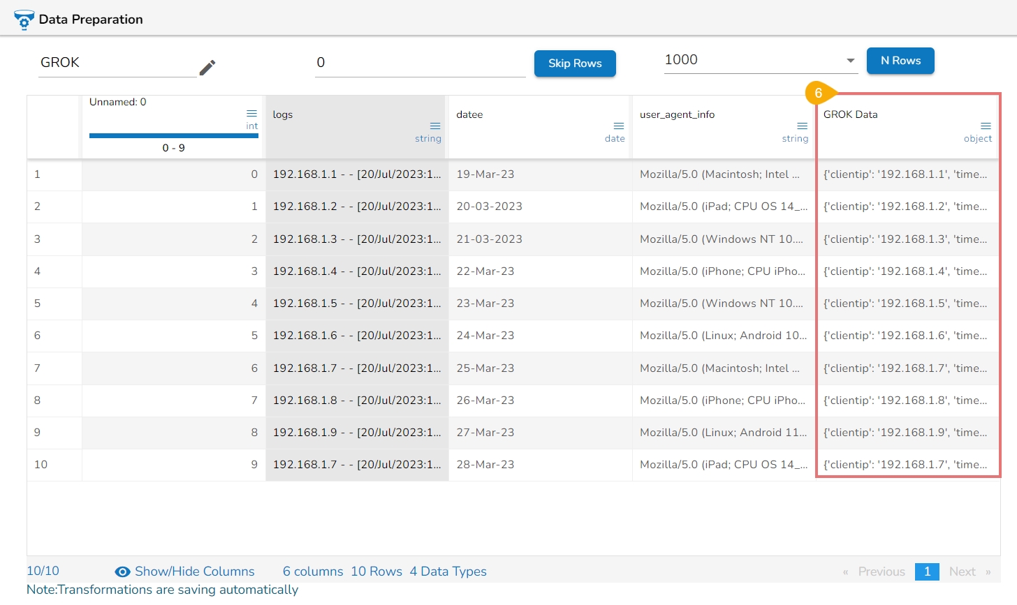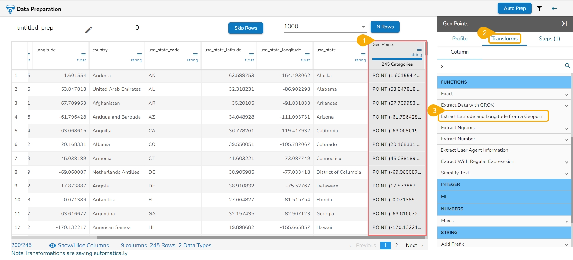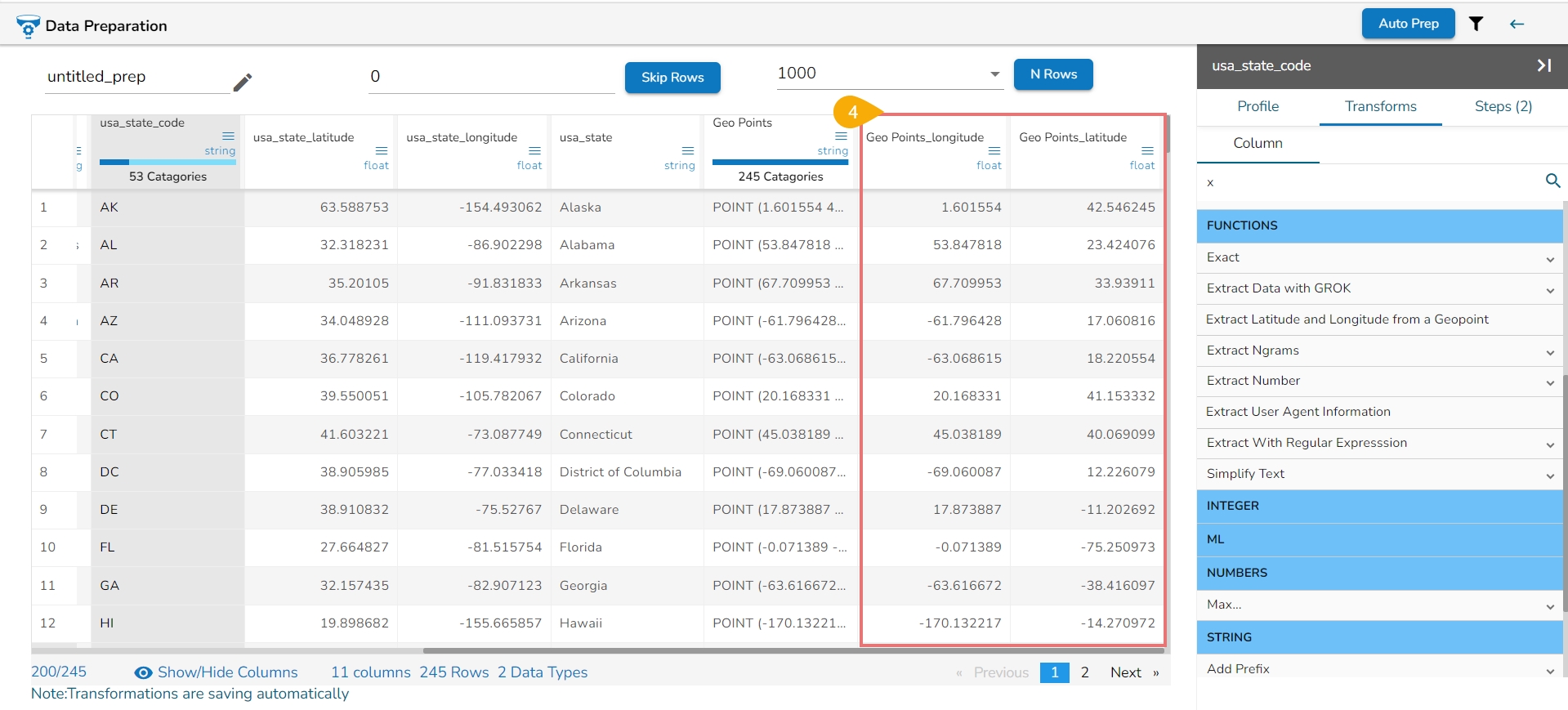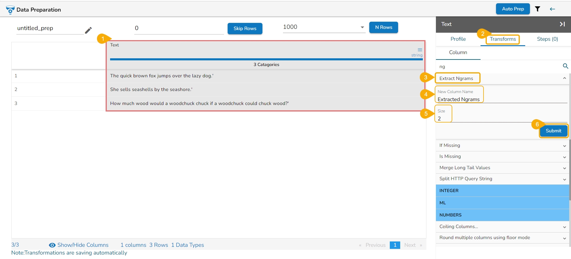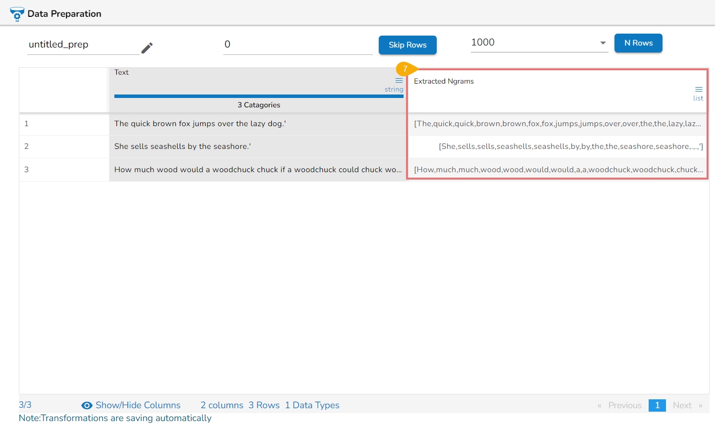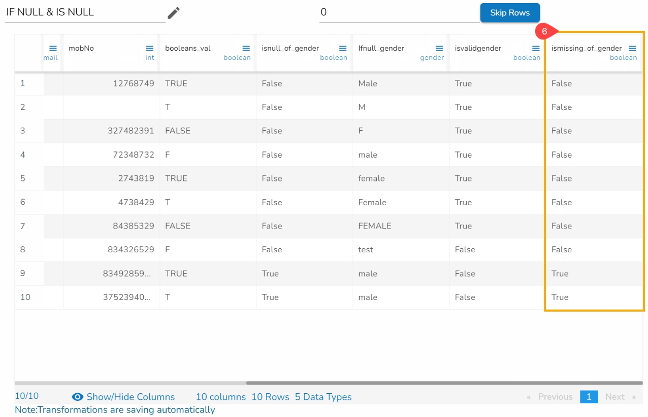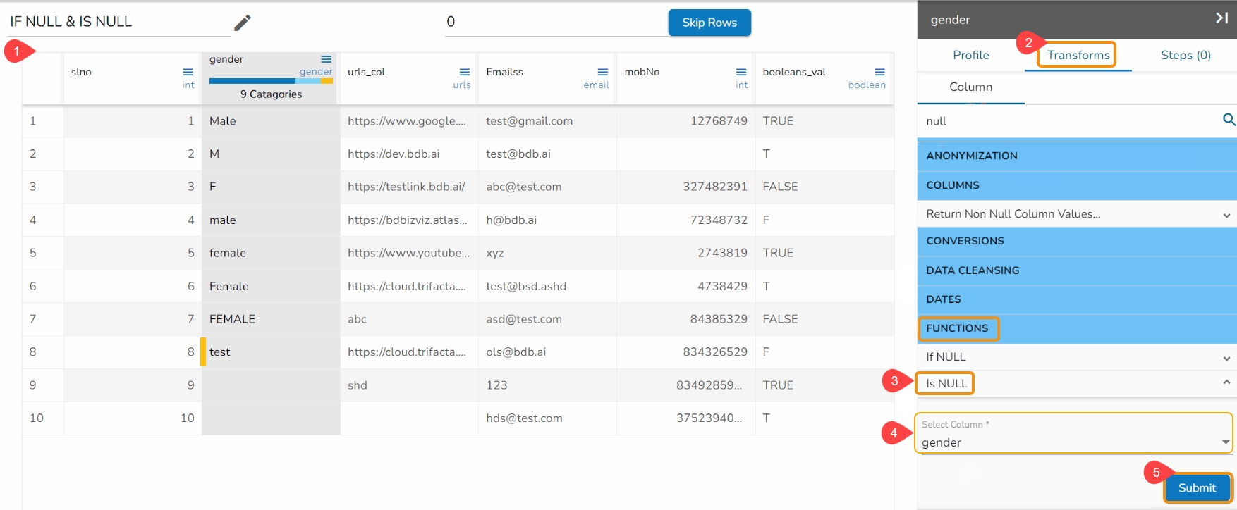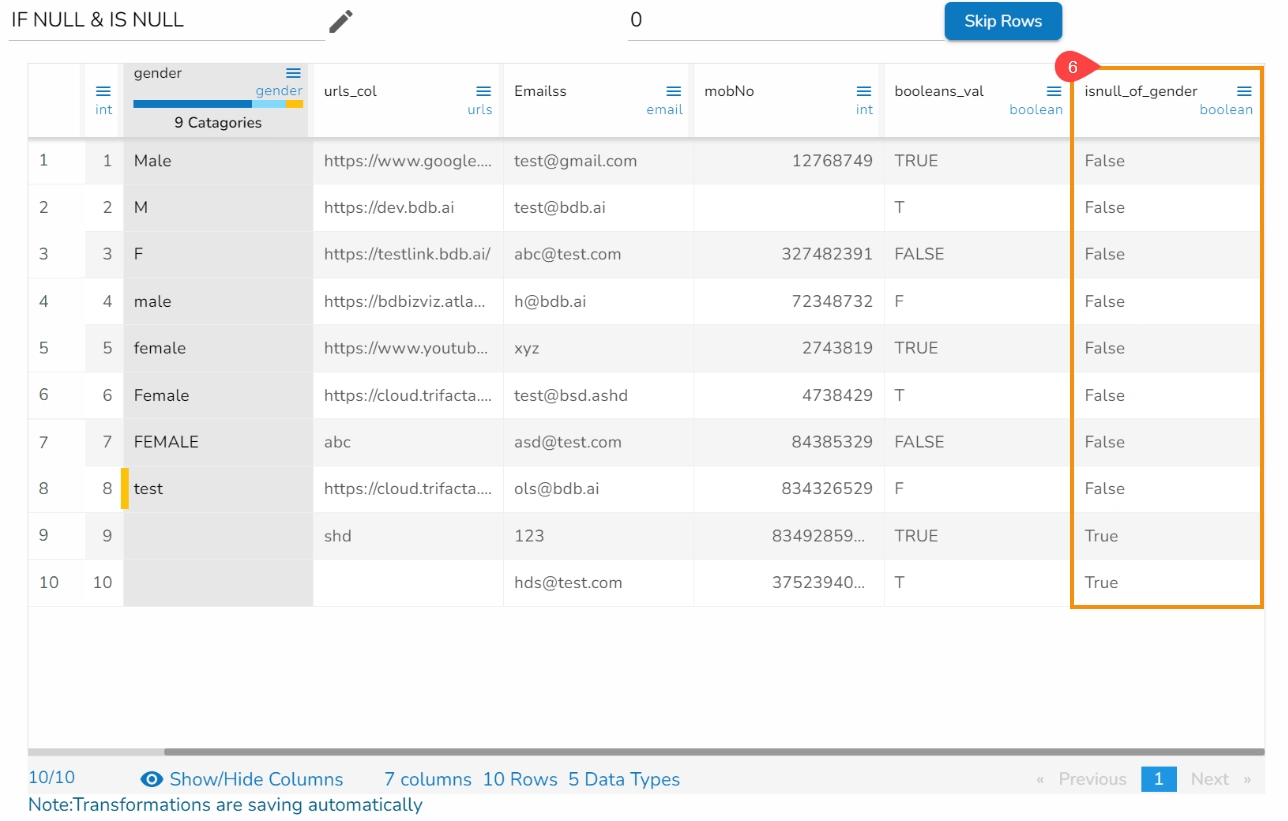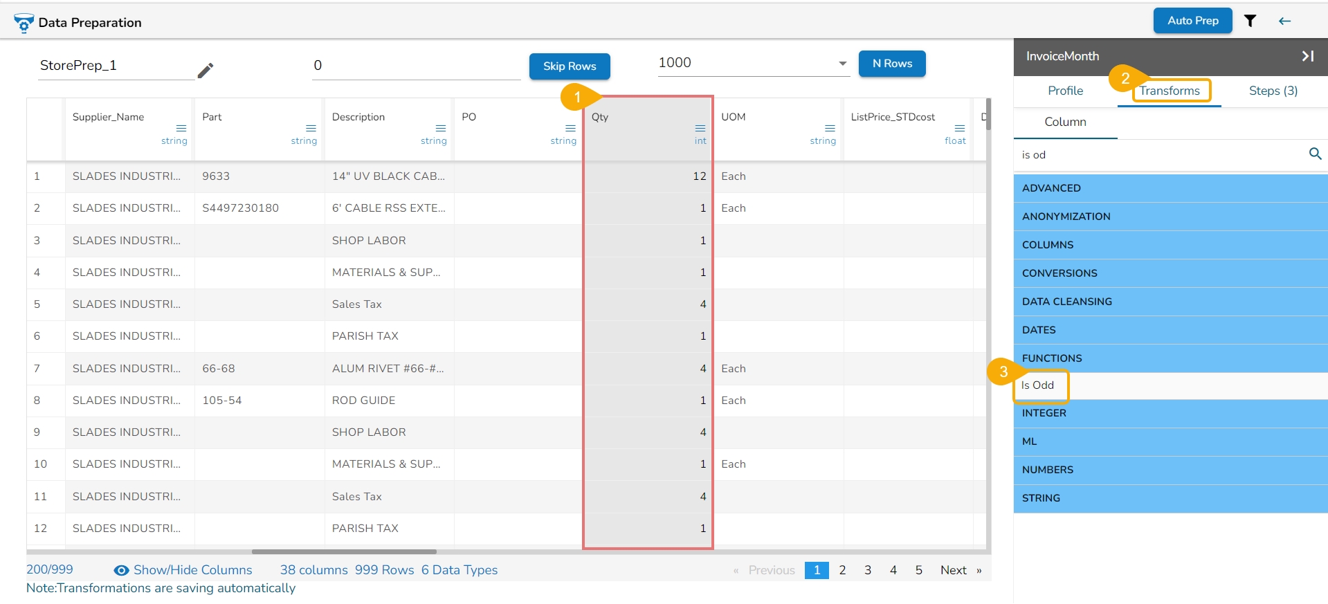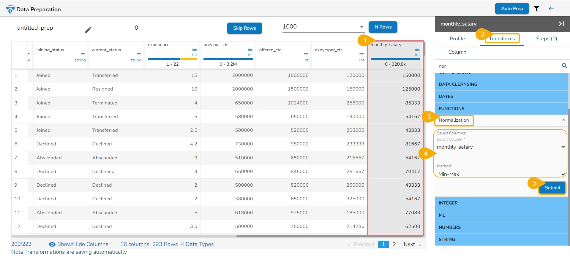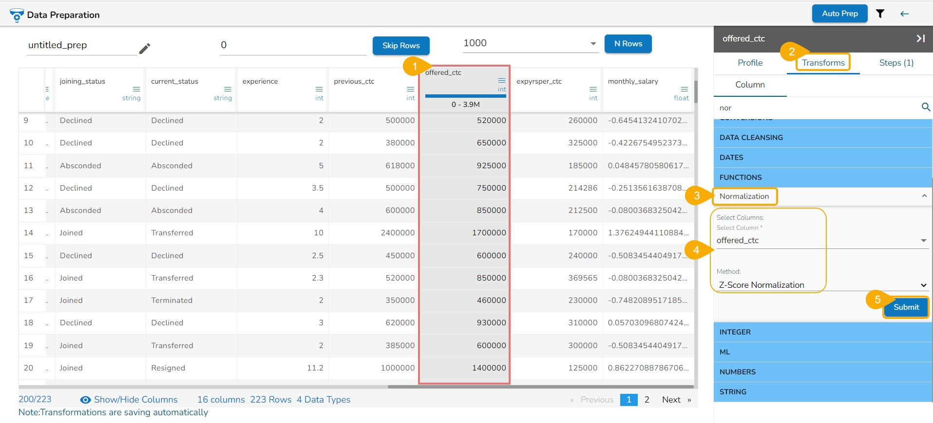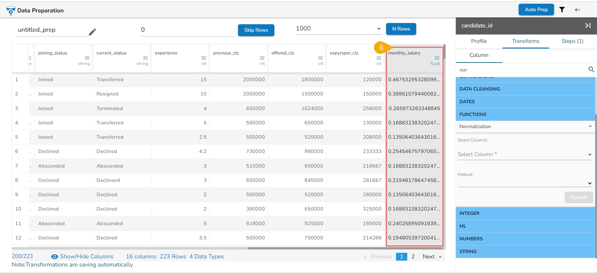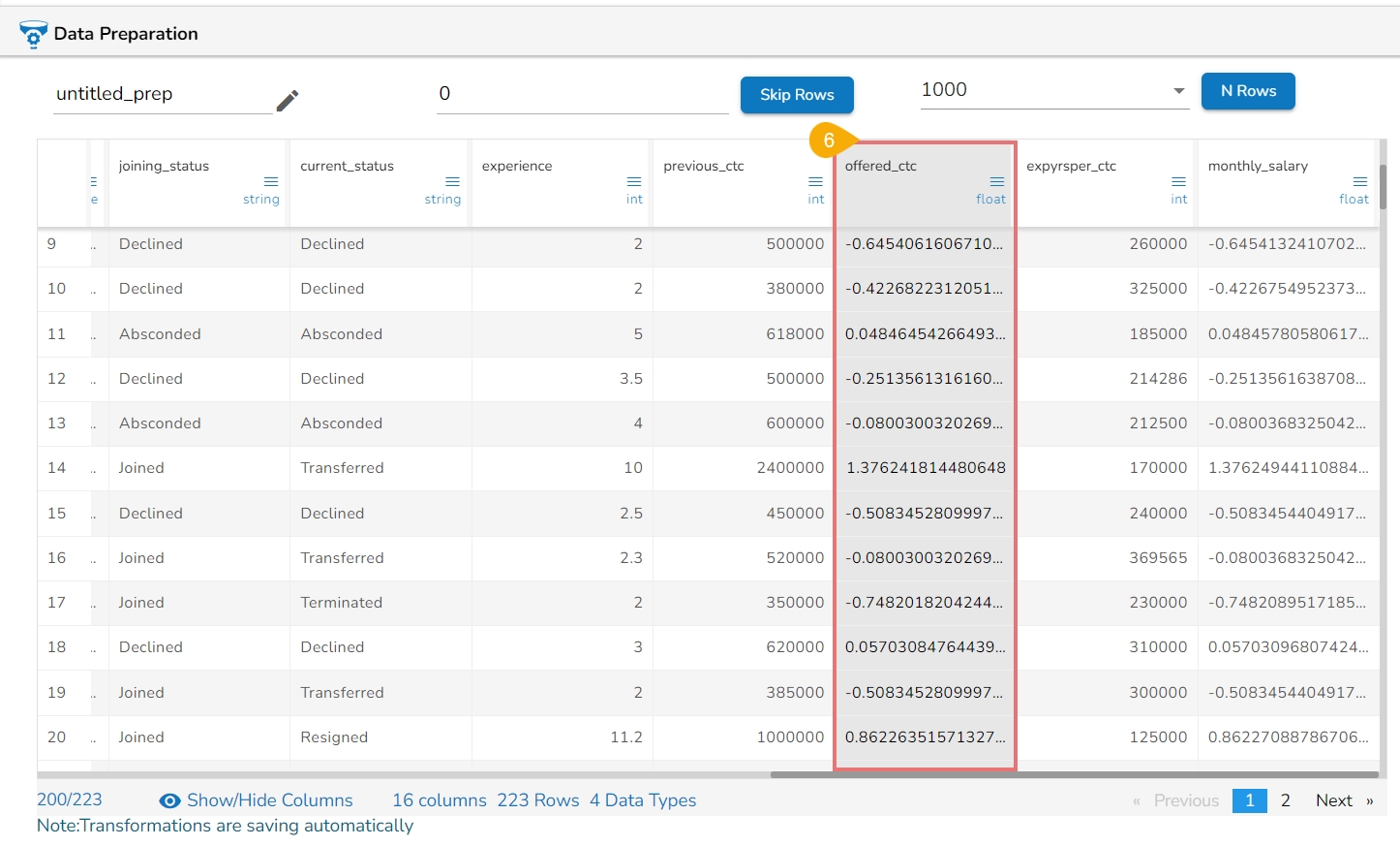
Loading...
Loading...
Loading...
Loading...
Loading...
Loading...
Loading...
Loading...
Loading...
Loading...
Loading...
Loading...
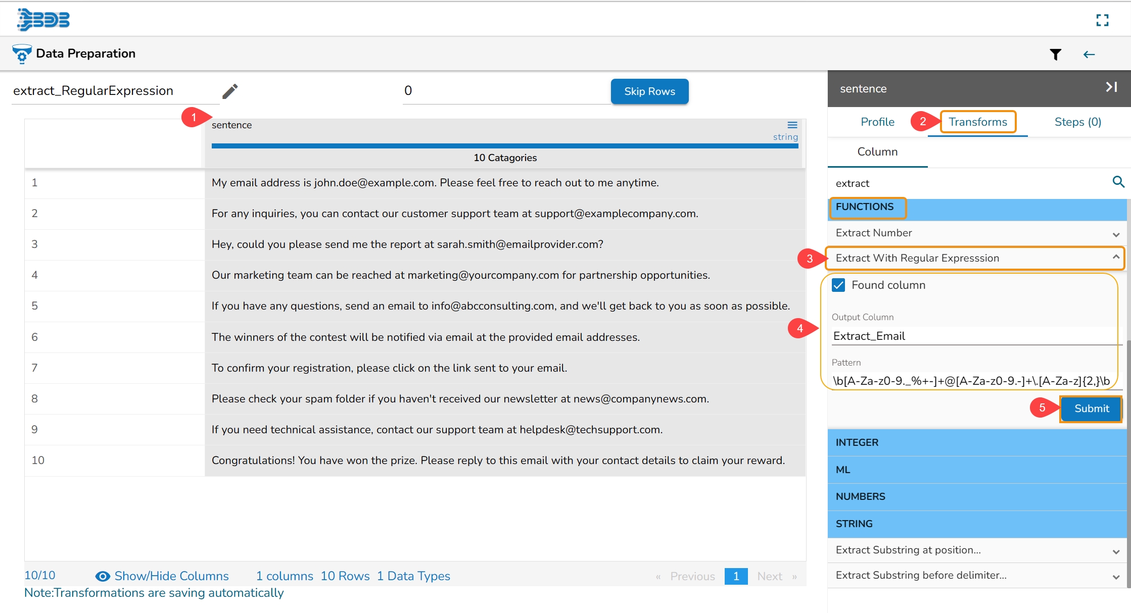
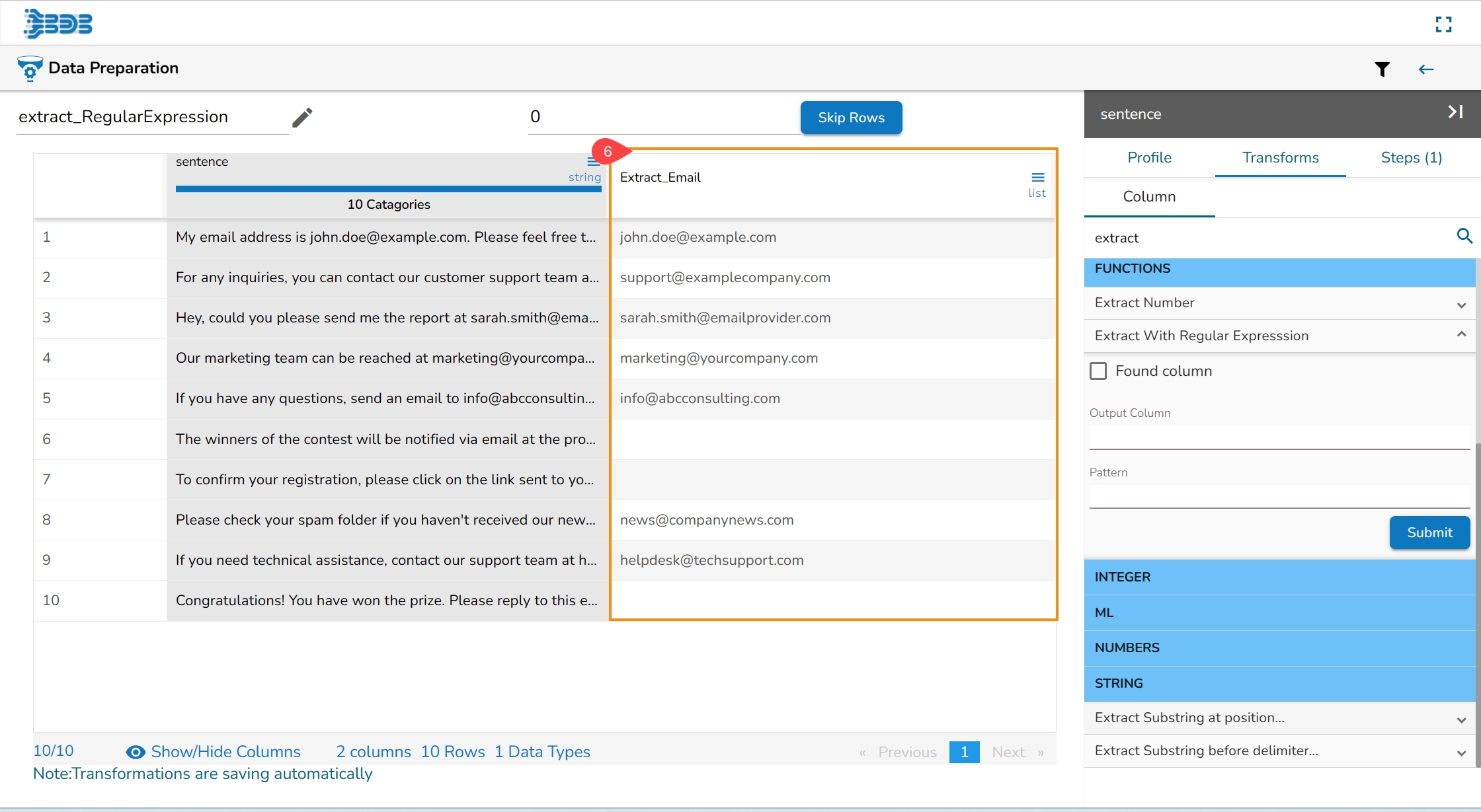
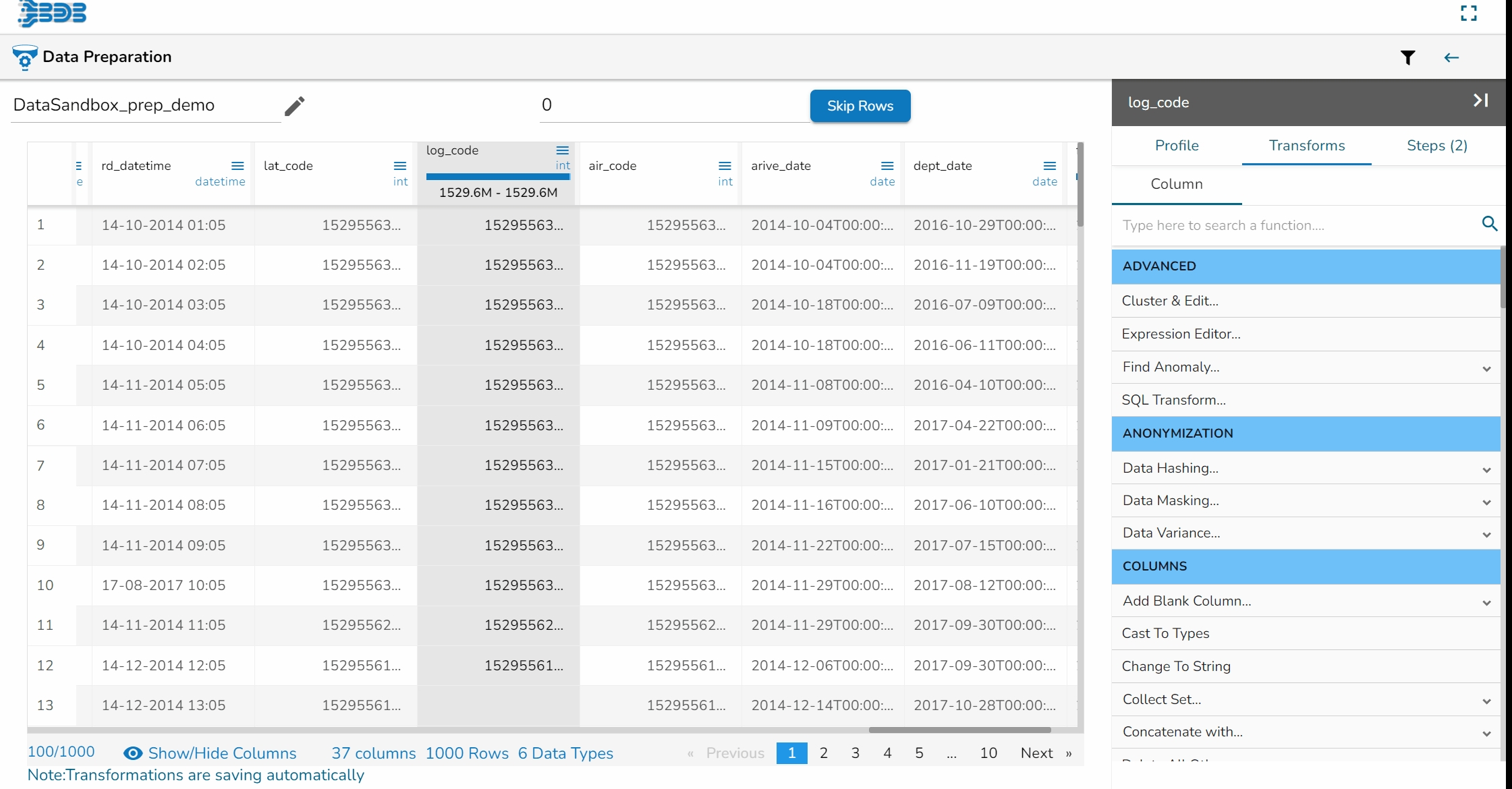
Find out the clusters based on the pronunciation sound and edit the bulk data in a single click.
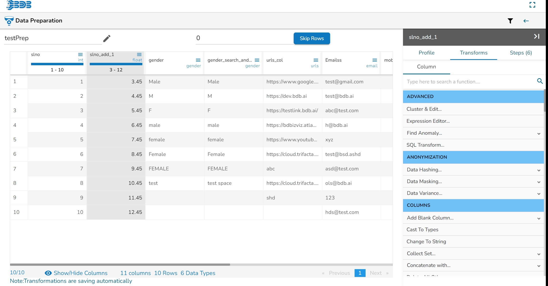
Check out the illustration on the Cluster & Edit transform.
Steps to perform the Cluster & Edit transform.
Select a column from the given dataset.
Open the Transforms tab.
Select the Cluster and Edit transform from the Advanced category.
The Cluster & Edit window opens.
The Method drop-down uses the Soundex phonetic algorithm for indexing names by sound as pronounced in English.
The Values found column lists number of values found from the data set related to a specific sound. E.g., In the given image the Values found display 5 categories.
The Replace Value column lists the anticipated replacements of the values found.
Select a value by using the checkbox that needs to be modified or changed. E.g., the 'tesi', 'test', and 'test3' are selected in the given example.
Search for a replace value or enter a value that you wish to be used as a replace value using the drop-down menu from the Replace Value column. For Example,
Click the Submit option.
The selected values from the column get modified in the data set.
This transform helps to execute expressions.
Check out the given illustration to understand the Expression Editor transform.
Steps to perform the Expression Editor transform:
Navigate to a Dataset within the Data Preparation framework.
Navigate to the Transforms tab.
Open the Expression Editor from the Advanced transforms.
The Expression Editor window opens displaying the following columns:
Functions: The first column contains functions for the user to search for a function. By using the double clicks on a function, it gets added to the given space provided for creating a formula.
Columns: The second column lists all the column names available in the selected dataset.
The Formula space is provided to create and execute various formulas/ executions. Click on a Formula name to get the expression on the right side
Use either of the following ways to consume the created expression or formula in the dataset.
Update a selected column by using the Update column option. The selected column will be updated with the chosen expression.
Create a new column with the created expression by selecting the Create a New Column option.
Provide a column name for the New Column.
Click the Submit option to either add a new column or update the selected column based on the executed formula/ expression.
The recently created or updated column with Formula gets added to the dataset.
Anomaly detection is used to identify any anomaly present in the data. i.e., Outlier. Instead of looking for usual points in the data, it looks for any anomaly. It uses the Isolation Forest algorithm.
Check out the given walk-through on the Find Anomaly transform.
Steps to perform the Find Anomaly transform:
Select a dataset within the Data Preparation framework.
Navigate to the Transforms tab.
Select the Find Anomaly transform from the ADVANCED category.
The Find Anomaly window opens.
Configure the following information:
Select Feature Columns: Select one or more columns where you want to find the anomaly.
Maximum Sample Size: The Isolation Forest algorithm takes the training data of a given sample size to find the normal value in the dataset.
Contamination (%): It is the percentage of observations we believe to be outliers. It varies from 0 to 1 (both inclusive).
Anomaly Flag Name: The result is either -1 or 1. 1 means the data is standard, and -1 means the data is an outlier. This information gets stored in the new column with the anomaly flag name.
Click the Submit option after the required details are provided.
The anomaly gets flagged under the column that has been named using the Anomaly Flag Name option.
Please Note: The other needed parameters such as Estimators and seed values are considered based on their default values to run the Isolation Forest logic on the selected dataset sample.
This transform helps to perform SQL queries. The user can customize the data with the
Check out the illustration on the SQL Transform.
Steps to perform the SQL transform:
Select a dataset within the Data Preparation framework.
Navigate to the Transforms tab.
Open the SQL Transform from the Advanced transforms.
The SQL Editor page opens displaying the Functions and Columns from the selected dataset.
Search a function and click it to get the default syntax suggestion in the text space and add it to the text space provided for writing a query.
Select the columns from the Columns list.
Write a query sentence with valid syntax by selecting an SQL function and related columns from the dataset. The displayed example may help to suggest a valid SQL query syntax.
Click the Submit option.
Please Note: Function syntax and small examples are displayed at the bottom of the window with the double-clicks on the function name.
The SQL query gets applied to the Data Set and based on the query the displayed dataset will be customized.
Please Note: The SQL Transform & Expression Editor supports only Pandas SQL Queries.
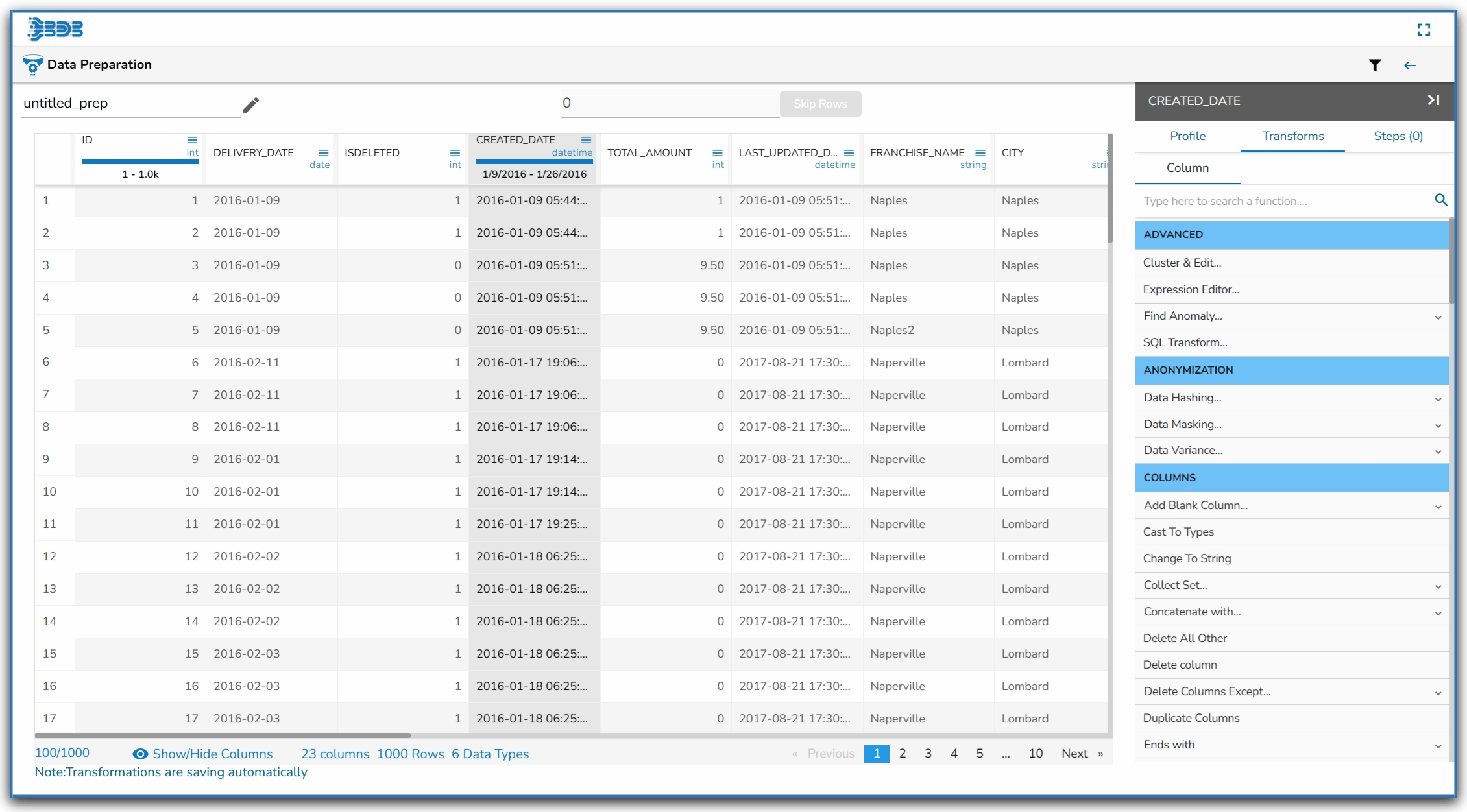
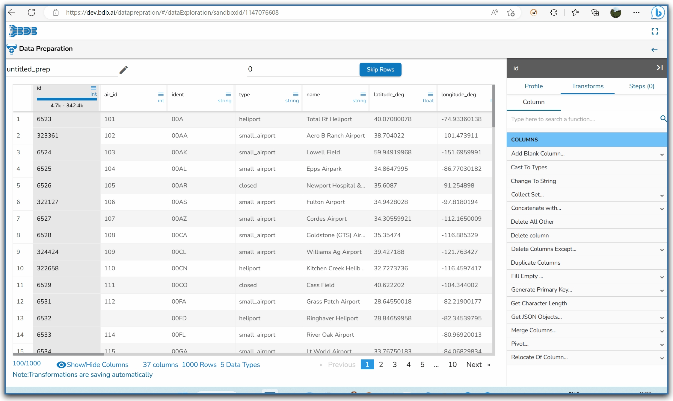
All the available Transforms are explained in this section. Please note that we are in process to update the UI changes for all the Transforms.
Anonymization is a type of information sanitization whose intent is privacy protection. It is a data processing technique that removes or modifies personally identifiable information.
The below-mentioned transforms are available under the Dates category:
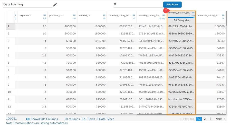
Data Hashing is a technique of using an algorithm to map data of any size to a fixed length. Every hash value is unique.
Data Hashing is a data transformation technique used to convert raw data into a fixed-length representation in the form of a hash value. This transformation is often employed as part of the data preprocessing stage before using the data for various purposes such as analysis, machine learning, or storage. The main objective of data hashing as a data transform is to provide a more efficient and secure way to handle and process sensitive or large datasets.
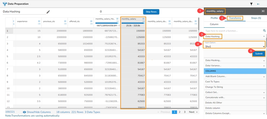
Check out the given illustration on how to use Data Hashing transform.
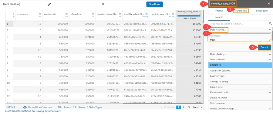
Steps to perform the Anonymization Transform:
Navigate to a dataset within the Data Preparation framework, and select a column.
Select one column that needs to be protected.
Select the Transforms tab.
Select the Data Hashing transform from the Anonymization category.
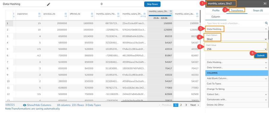
The Data Hasing window opens.
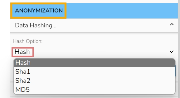
Use the drop-down menu to get the available hashing options.
Select a Hash option (E.g., Sha2 hash option has been selected).
Set the Hash Value using the drop-down menu. The default Hash Value is 256 for the Sha2 hash option.
Click the Submit option.
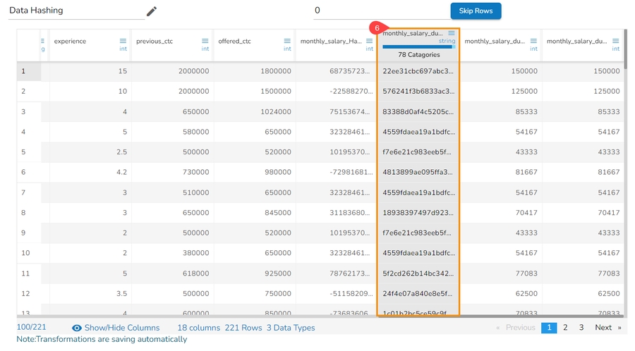
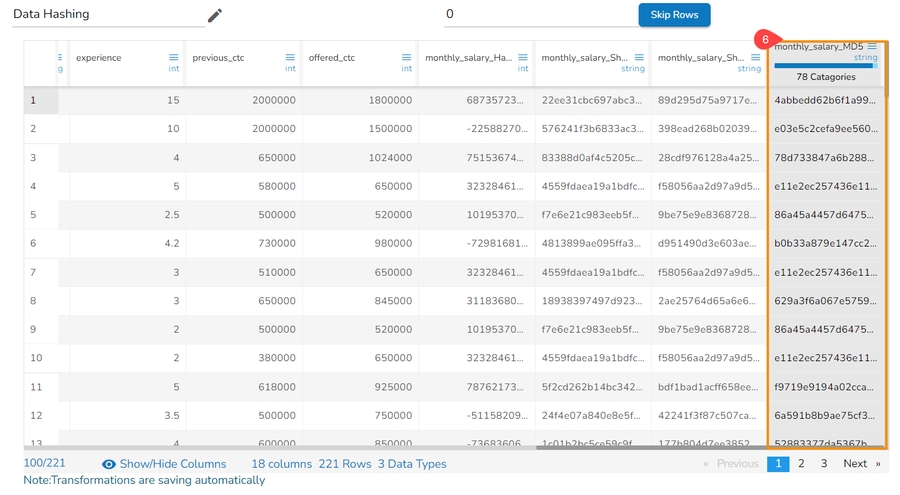
Data in the selected column will be transformed using the hashed format.
Please Note:
A suitable hashing algorithm is chosen based on the specific requirements and security considerations as Hash Options. The supported Hash options are Hash, Sha-1, Sha-2, and MD-5.
The hash options displayed in the UI map to the following actual hashing algorithms on the backend:
Sha1 (UI) → SHA-256 (Backend)
Sha2 (UI) → SHA-512 (Backend)
Hash (UI) → MD-5 (Backend)
MD5 (UI) → MD-5 (Backend)
Data masking transform is the process of hiding original data with modified content. It is a method of creating a structurally similar but inauthentic version of actual data.
Check out the given walk-through on the Data Masking transform.
Steps to perform the Data Masking Transform:
Navigate to a dataset within the Data Preparation framework, and select a column.
Select one column that needs to be protected.
Select the Transforms tab.
Select the Data Masking transform from the Anonymization category.
The Data Masking dialog box opens.
Provide the Start Index and End Index to mask the selected data.
Click the Submit option.
The image displays how the Data Masking transform (when applied to the selected dataset) converts the selected data:
The Data Variance transform allows the users to apply data variance to the Numeric and Date columns.
Check out the illustration on how to use the Data Variance on a numeric column.
Select a numeric column within the Data Preparation framework.
Open the Transforms tab.
Select the Data Variance transform from the Anonymization category.
The Data Variance dialog box opens.
Configure the following information:
Select Numeric as the Value Type.
Select an Operator using the drop-down option.
Set percentage.
Provide a comment in the given section.
Click the Submit option.
The data of the selected column gets transformed based on the set of numeric values.
Check out the illustration on how to use the Data Variance on a date column.
Select a column containing Date values from the given dataset within the Data Preparation framework.
Open the Transforms tab.
Select the Data Variance transform from the Anonymization category.
The Data Variance dialog box opens.
Configure the following information:
Select Date as the Value Type.
Select an Input Format from the drop-down list.
Select a Start Date using the Calendar option.
Select an End Date using the Calendar option.
Provide a comment in the given section.
Click the Submit option.
The selected Date column will display random dates from the selected date range.
Please Note: The Data Variance transform also provides space to add description while configuring the transformation information.
This transformation using the Salt and Pepper technique is a method to protect sensitive data by introducing random noise or fake data points into a dataset while preserving its statistical properties.
Check out the illustration on the Hashing Anonymization transform.
Navigate to a dataset within the Data Preparation framework, and select a column.
Select one column that needs to be protected.
Select the Transforms tab.
Select the Hashing Anonymization (using salt & pepper technique) transform from the Anonymization category.
The Hashing Anonymization (Using the salt & pepper technique) dialog window opens.
Provide a value using the Set Values space.
Select a field using the Set Fields drop-down menu.
Select a hashing option using the Hash Option drop-down menu.
Click the Submit option.
The target column data will be displayed after applying the selected hashing option.
Please Note:
The first user-provided value (entered in the "Set Values" field) acts as the pepper.
Selected column values will act as the salt.
The hash options displayed in the UI map to the following actual hashing algorithms on the backend:
Sha1 (UI) → SHA-256 (Backend)
Sha2 (UI) → SHA-512 (Backend)
Hash (UI) → MD-5 (Backend)
MD5 (UI) → MD-5 (Backend)
The transform converts any duration (day, hour, minute, seconds, or milliseconds) to any specified duration.
To perform the transform, select the column that has the duration to be converted and specify the duration type.
Check out the given illustration on how to apply Convert Duration.
Navigate to the Data Preparation workspace.
Select a column from the data set with the time duration.
Open the Transforms tab.
Select the Convert Duration transform from the Conversion category.
The Convert Duration dialog box appears.
Provide the following information to apply the convert duration transformation.
Enable the Create New Column option to create a new column.
From: The type of source interval
To: The type of destination interval
Precision: The decimal points to be retained.
Click the Submit option.
The selected column values transform to align with the chosen conversion duration. For instance, in this scenario, the selected column values undergo a conversion, transitioning from the unit of days to hours.
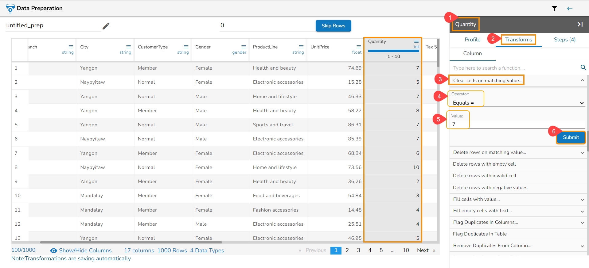
Clear the cell value on matching the condition specified. Operators include contains, equals, starts with, end with, and regex match. Transform applies in the same column.
The Clear Cells on Matching Value data transform is a process used to remove or delete the contents of specific cells in a dataset or spreadsheet based on a given condition or matching value. This transformation is commonly employed to clean or manipulate data by selectively clearing cells that meet certain criteria.
Here's an overview of how the Clear Cells on Matching Value data transform works:
Select a column.
Navigate to the Transforms tab.
Select the Clear Cells on Matching Value transform from the Data Cleansing category.
Operator: Select the operator required for matching from the list.
Value: The value or pattern to be searched for in the selected column.
Click the Submit option.
Please Note: The supported Operators for this Transform are: equals, starts with, end with, and regex.
The value selected in the Quantity column clears the cell with 0 value.
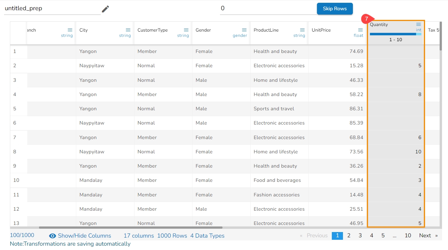
It removes the values from the cells with 7 value and returns blanks cells:
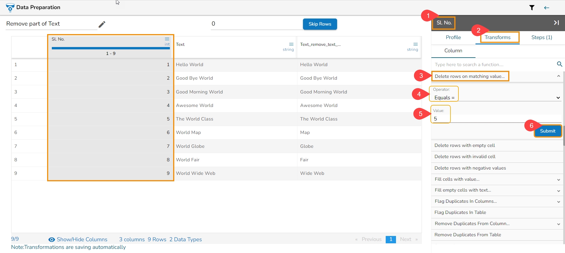
Delete the rows on matching the condition specified for that column.
The Delete Rows on Matching Value transform is a data manipulation process used to remove rows from a dataset based on a specified condition or matching value. This transformation allows the user to selectively delete rows that meet certain criteria.
Here's an overview of how the Delete Rows on Matching Value transform works:
Select a column.
Navigate to the Transforms tab.
Select the Delete Rows on Matching Value transform from the Data Cleansing category.
Operator: Select the operator required for matching from the list.
Value: The value or pattern to be searched for in the selected column.
Click the Submit option.
Please Note: The supported operators are: contains, equals, starts with, ends with, and regex match.
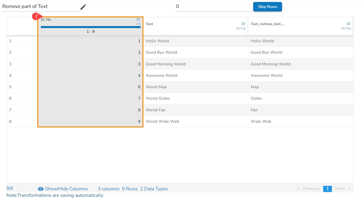
The row with given value from the Sl. No. column gets deleted.
The row with 5 value has got deleted from the id column.
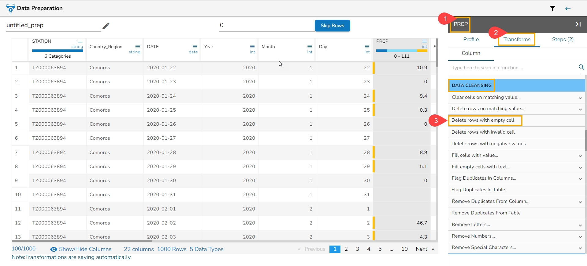
The Delete Rows with Empty Cell transform is a data manipulation operation commonly used in spreadsheet software or data processing tools to remove rows that contain empty cells within a specified column or across multiple columns. The transform helps clean and filter data by eliminating rows that lack essential information or have incomplete records.
Select a column.
Navigate to the Transforms tab.
Click the Delete Rows with Empty Cell transform from the Data Cleansing category.
Please Note: This transform does not have a form to configure, it gets applied by clicking the transform name.
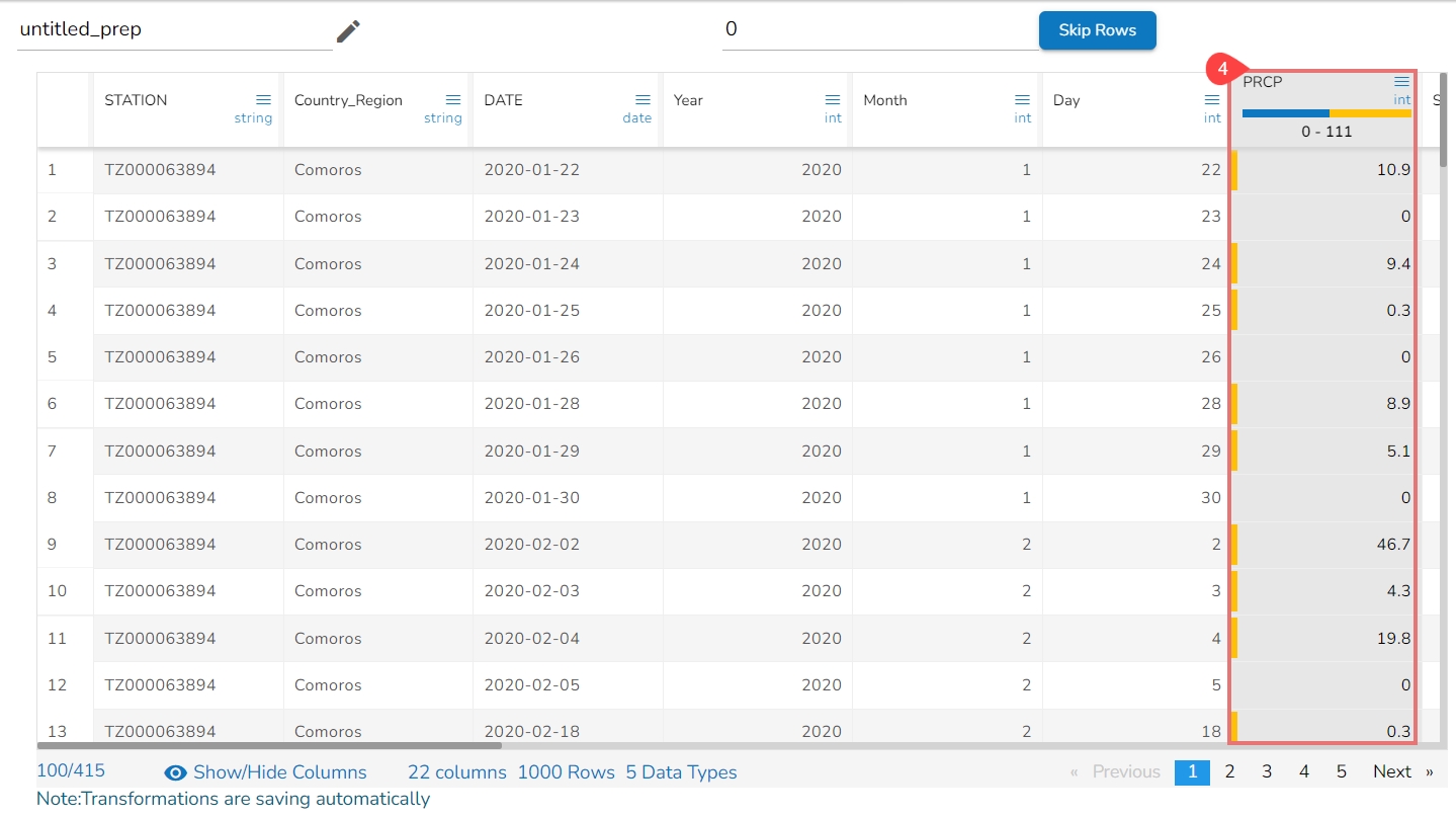
It deletes all the rows with empty cell in that column returning the data as below:
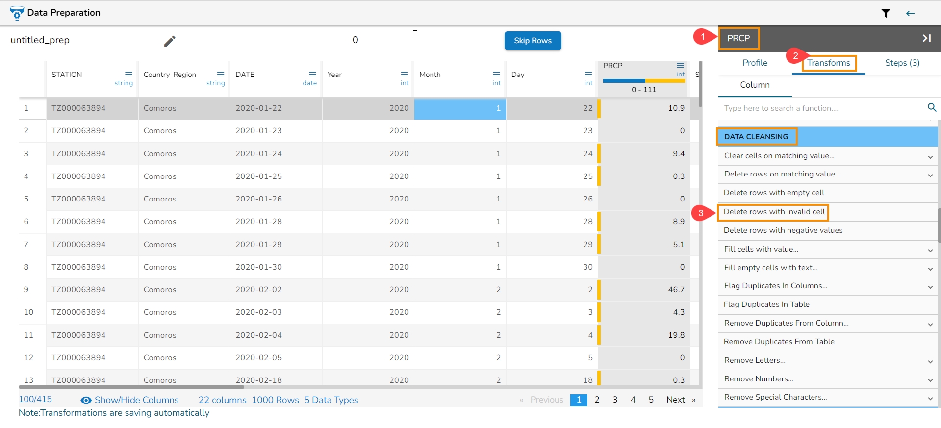
The Delete Rows with Invalid Cell transform is a data manipulation operation used to remove rows that contain invalid or inconsistent data in a specified column or across multiple columns. This transform helps clean and filter data by eliminating rows that do not meet specific validation criteria or fail to comply with predefined rules.
Refer to the following steps on how the Delete Rows with Invalid Cell transform works:
Select a column.
Navigate to the Transforms tab.
Select the Delete Rows with Invalid Cell transform from the Data Cleansing category.
Please Note: This transform does not have a form to configure, it gets applied by clicking the transform name.
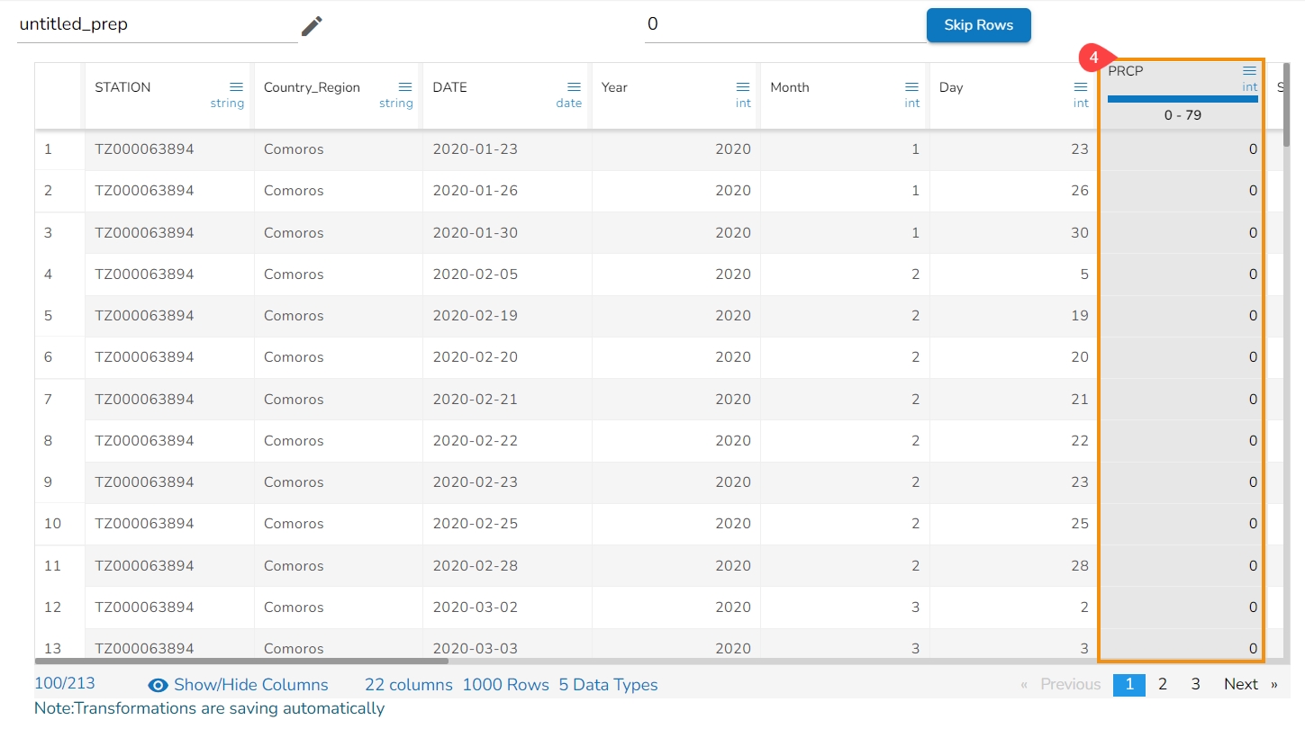
The transform deletes rows with an invalid value in the selected column.
The Delete Rows with Negative Values transform is a data manipulation operation used to remove rows that contain negative values in a specified column. This transform helps to filter and clean data by eliminating rows that have undesired negative values.
Select a column.
Navigate to the Transforms tab.
Select the Delete Rows with Negative Values transform from the Data Cleansing category.
Please Note: This transform does not have a form to configure, it gets applied by clicking the transform name.
It deletes the row with the negative value and returns the data as displayed below:
The Fill Cells with Value transform is a data manipulation operation used to replace empty or missing cells with a specified value in a column or across multiple columns. This transform helps to ensure data consistency and completeness by filling in gaps or replacing missing values.
Select a column.
Navigate to the Transforms tab.
Select the Fill Cells with Value transform from the Data Cleansing category.
Use with: Specify whether to fill with a value or another column value
Column/ Value: The value with which the column must be filled, or the column with which the value must be replaced. When the above transform is applied to the below data on the column timecol2, it fills the column with the selected value that is 30.
Click the Submit option.
Please Note: The user can also fill the column value with another column's values if the selected option is Column. E.g., the following image mentions the values of the timecol3 is provided for the timecol2.
It fills the selected column with a value or a value from another column.
It helps to fill the empty cells of a selected column with a value or a value from another column if the destination column is empty.
Select a column.
Navigate to the Transforms tab.
Select the Fill Empty Cells with Text transform from the Data Cleansing category.
Use with: Specify whether to fill with a value or another column value.
Column/ Value: The value with which the column must be filled, or the column with which the value must be replaced.
Click the Submit option.
When the transform is applied to the below data on the empty cell of the Bol column,
It fills the empty cell with the chosen text:
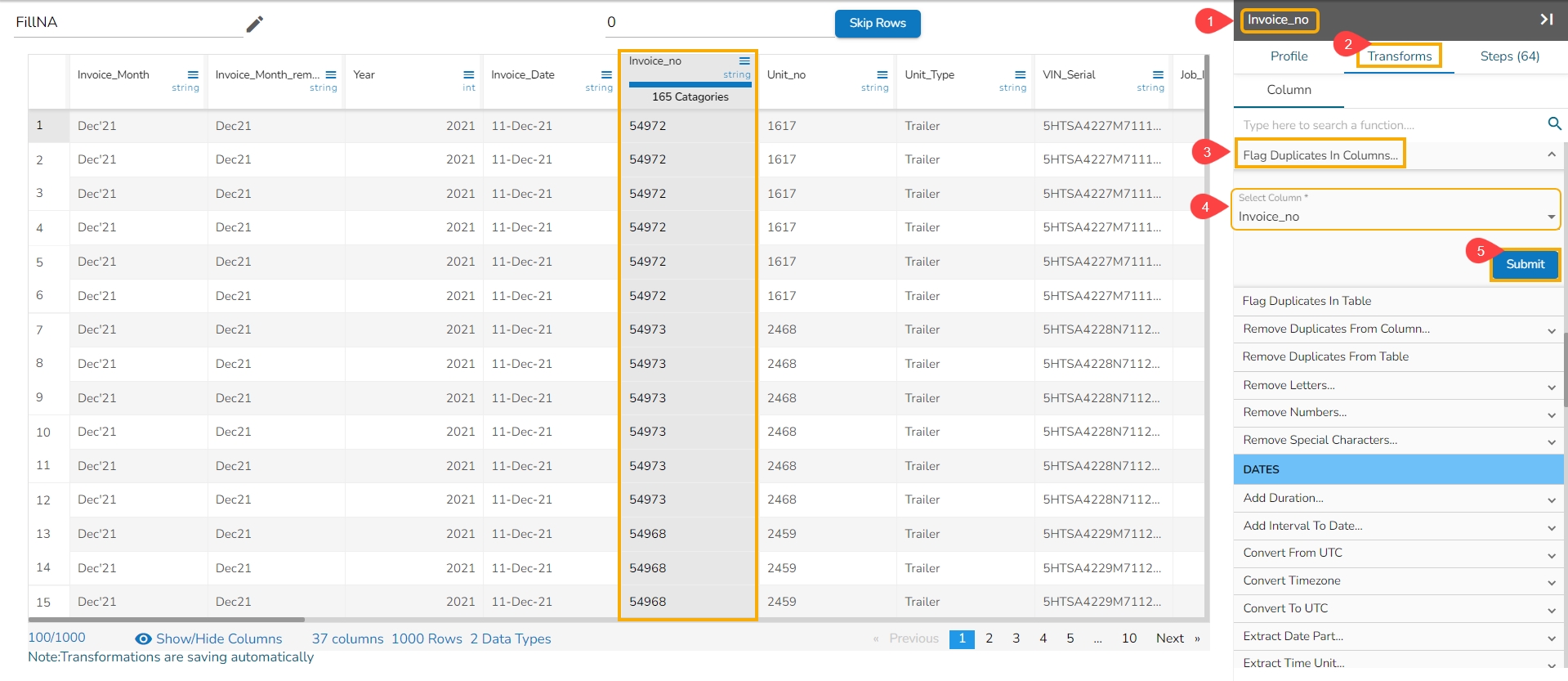
This transform adds a new Boolean column based on duplicate values in the column. For original value it gives false, and for the duplicate value, it provides true value.
Select a column.
Navigate to the Transforms tab.
Select the Flag Duplicates in Columns transform from the Data Cleansing category.
Select the column that contains duplicate values.
Click the Submit option.
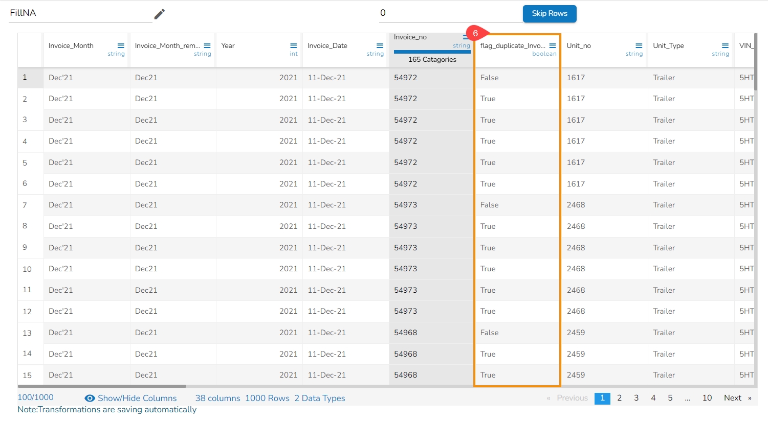
It inserts a new column by flagging the duplicated values as true.
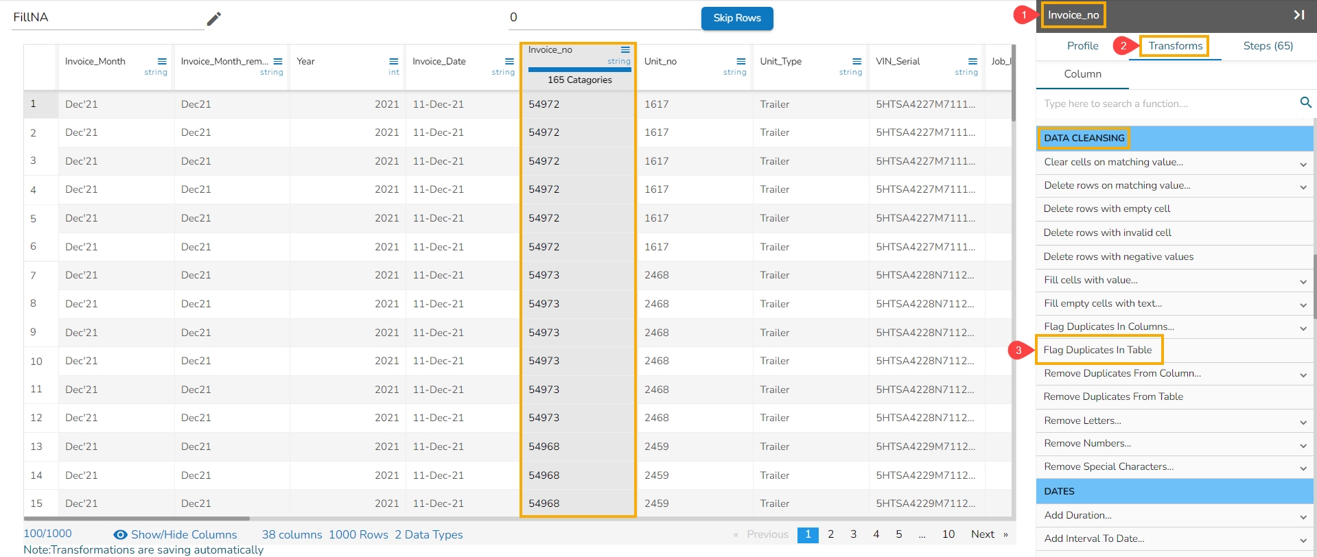
This transform adds a new Boolean column based on duplicate rows in the table. For original value it gives false, and for the duplicate value, it provides true value.
Select a column that contains duplicate values.
Navigate to the Transforms tab.
Click the Flag Duplicates in Table transform from the Data Cleansing category.
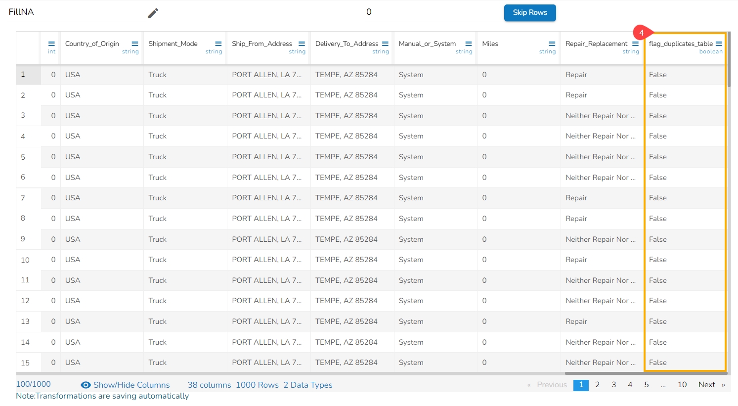
When applied on a column it inserts a new column named with the 'flag_' prefix and mentions the duplicated values as true.
The duplicated values get notified as true in the flag_duplicates_table column.
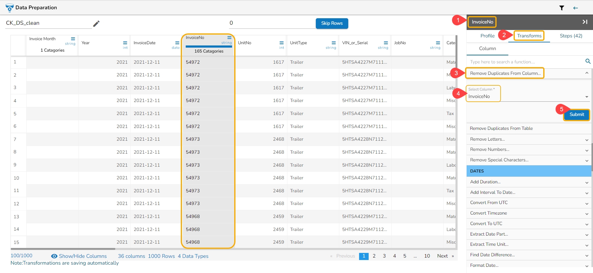
It removes duplicate values from the selected columns. This transform can be performed on a single as well as on multiple columns.
Select a column.
Navigate to the Transforms tab.
Select the Remove Duplicates from Column transform from the Data Cleansing category.
Select the column that contains duplicate values.
Click the Submit option.
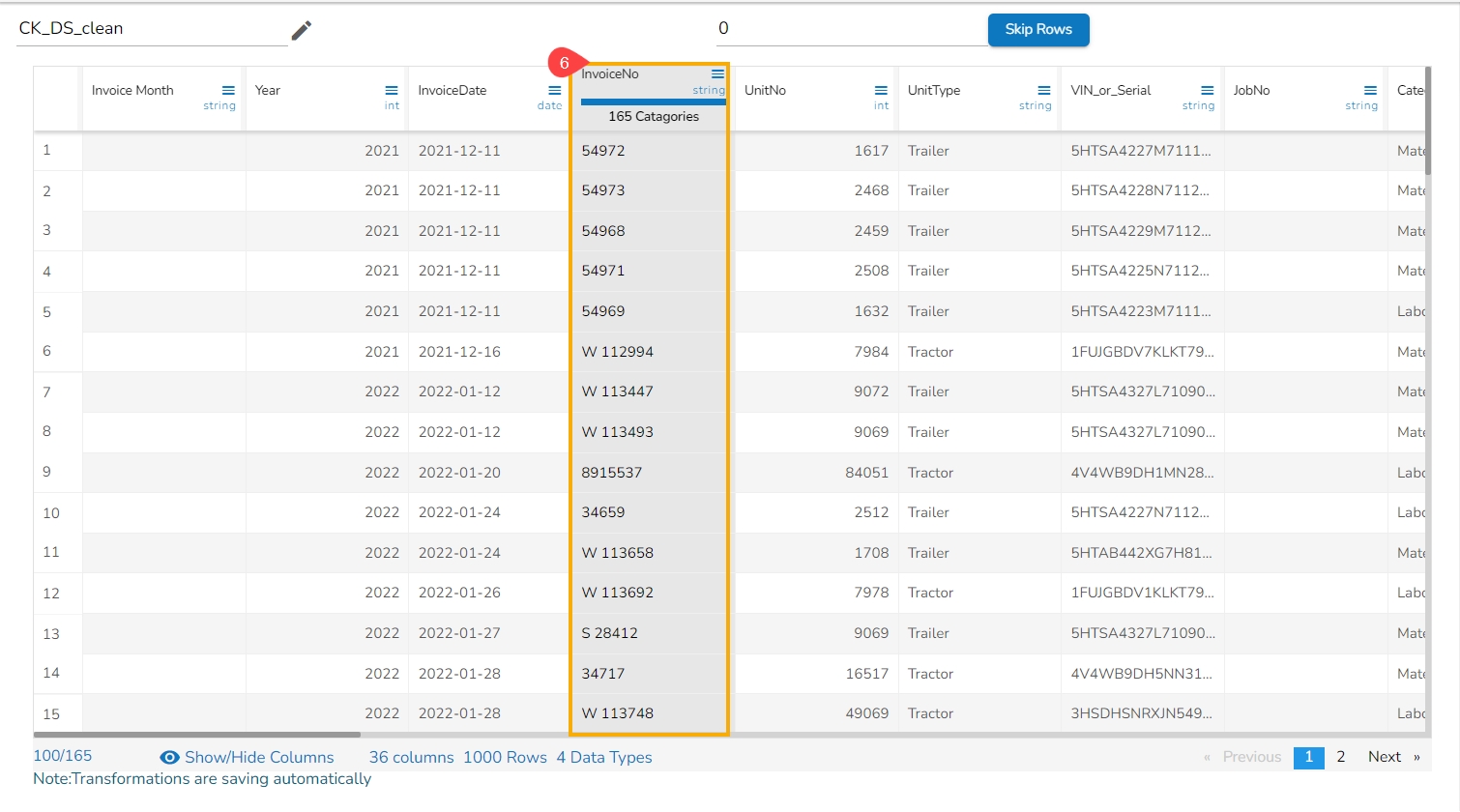
The duplicated values get removed from the column.
It removes all duplicate rows from the table.
Select a column.
Navigate to the Transforms tab.
Select the Remove Duplicates from Table transform from the Data Cleansing category.
The duplicated data from the selected column gets deleted.
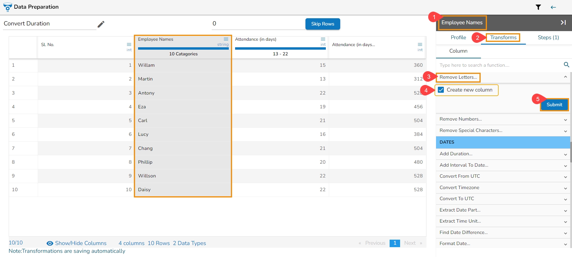
It removes any letter present in the selected column. The users can either add a new column with the transformed value or overwrite the same column.
Select a column.
Navigate to the Transforms tab.
Select the Remove Letter transform from the Data Cleansing category.
Enable create new column to create a new column with the transform result.
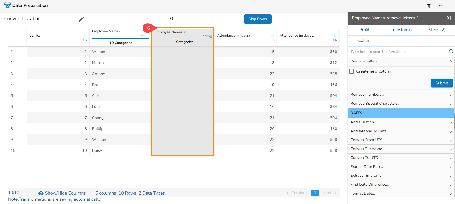
Click the Submit option.
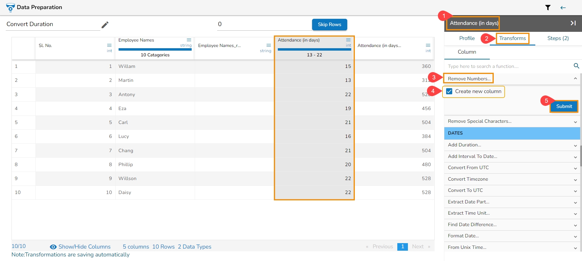
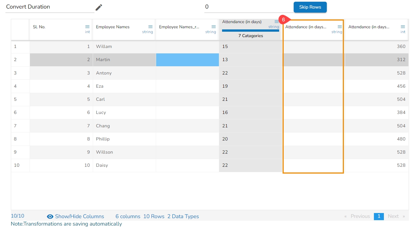
It removes the numbers from the newly inserted column.
It removes any number present in the selected column. We can either add a new column with the transformed value or overwrite the same column.
Select a column.
Navigate to the Transforms tab.
Select the Remove Letter transform from the Data Cleansing category.
Enable create new column to create a new column with the transform result.
Click the Submit option.
When the Remove Numbers, transform gets performed on a selected column,
It removes numbers from the selected column.
This transform helps to remove the special characters from the metadata (column headers) of a dataset & make it useful in other modules.
Check out the given illustration on how to Remove Special Characters from Metadata.
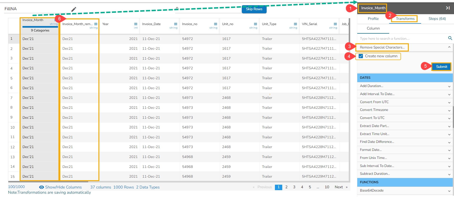
It removes any special character present in the selected column. Only letters, numbers, and spaces are retained. We can either add a new column with the transformed value or overwrite the same column.
When the transform Remove Special Characters gets performed on the selected column, the punctuations get removed from the column.
Select a column.
Navigate to the Transforms tab.
Select the Remove Special Characters transform from the Data Cleansing category.
Enable the Create new column option.
Click the Submit option.
The special character gets removed from the newly added column.
This transform removes leading and trailing quotes from a text. It can be applied to both single quotes (') and double quotes (").
Steps to perform the transform:
Navigate to the Data Preparation landing page.
Select a String datatype Column where single or double quotes in the values as trail & lead part.
Open the Transform tab.
Navigate to the Data Cleansing transform type.
Click the Remove Trail and Lead Quotes transform.
As a result, the quotes will get removed and changes will be reflected in the same source column.
This transform removes Trail and all Whitespaces found at the beginning and end of the text.
Steps to perform the transform:
Select a String datatype Column where whitespace is present in the values as trail & lead part.
Click on the Remove trail and lead whitespace transform.
Whitespace will get removed from the trail and lead places and changes will be reflected in the same source column.
This transforms removes all whitespace from a string, including leading and trailing whitespace and all whitespace within the string.
Steps to perform the transform:
Navigate to the Data Preparation landing page displaying the Data.
Select a String datatype Column where whitespace is present in the values as trail, between & lead part.
Open the Column
Click the Remove Whitespace transform.
Use checkbox to select the Create New Column option.
Provide a name for the New Column.
Click the Submit option.
Whitespace will get removed from the lead, in-between, and trail spaces of the content of the source column and displayed as a new column in the data set.
The users can avoid creating a new column while using the Remove Whitespace transform in that case, the whitespaces will get removed from the source column itself.
The transform adds two-time values. It can either add the selected column with a time value or time from another column.
Please Note: The transform supports adding time into ‘hh:mm:ss.mmm’ and ‘hh:mm:ss’ formats.
Use with: Specify whether to fill with a value or another column value
Column/ Value: The value with which the column must be added, or the column with which the selected column value must be added.
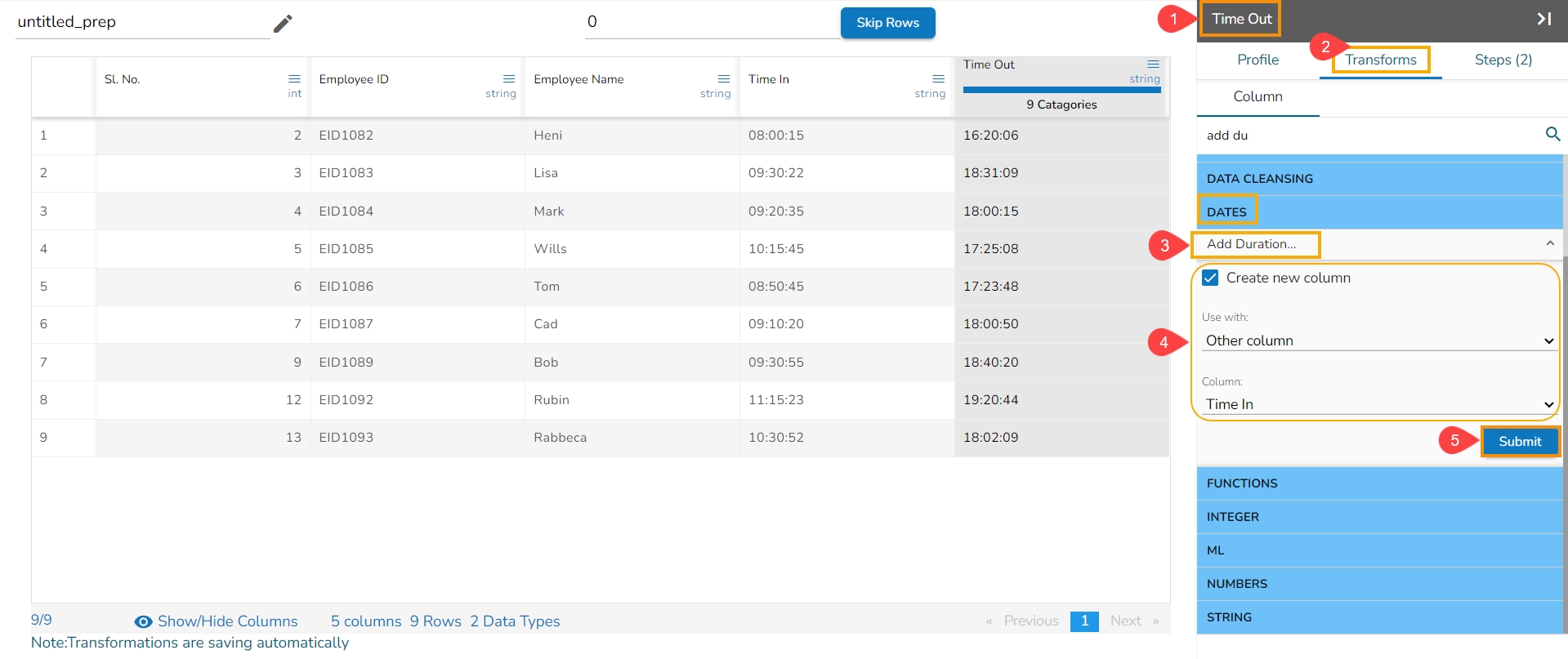
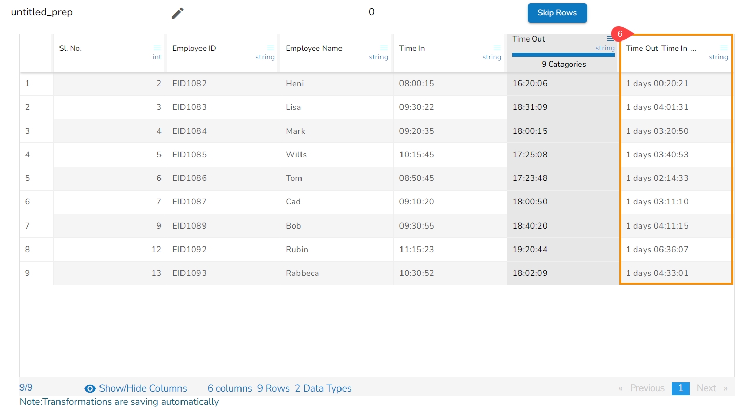
The Add Duration transform is applied to the timecol2, and the selected other column is timecol3 to configure the transform:
Select a column with the time values (In this case, the selected column is Time Out).
Open the Transforms tab.
Select the Add Duration transform from the Date transform category.
Enable the Create new column option, if you wish to display the transformed data in a new column.
Select the Other Column option from the drop-down option.
Select another column using the drop-down option from where the duration values are to be counted (In this case, the selected column is Time In column).
Click the Submit option.
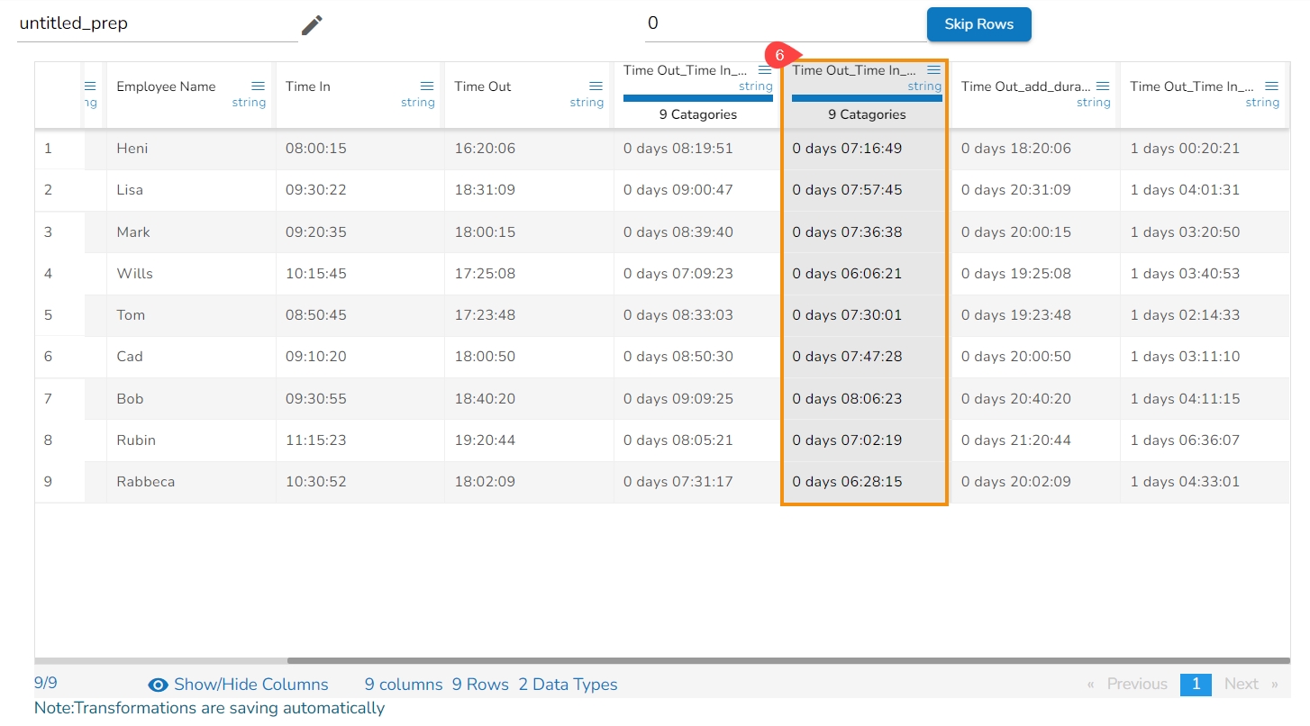
A new column gets created displaying the duration values as displayed below:
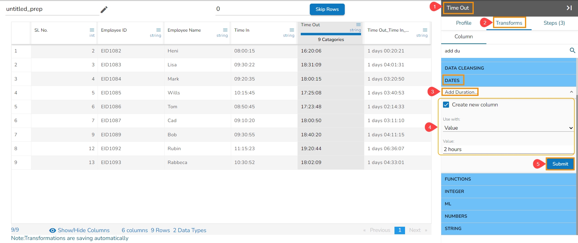
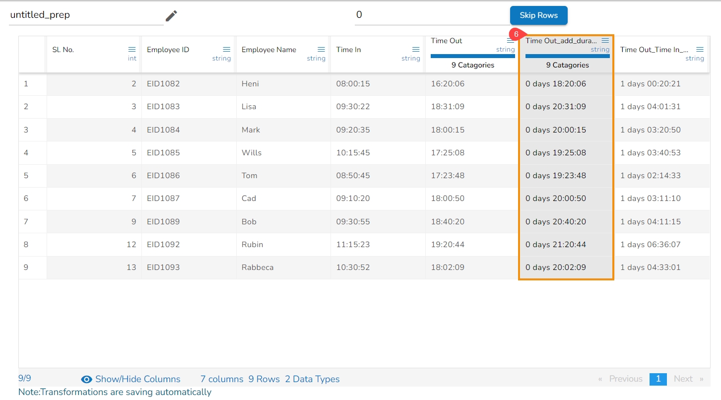
The Add Duration transform has been applied to the Time Out column with Value option where in the set value is 2 hours.
A new column gets added to the Data Grid displaying duration based on the set value as shown in the below-given image:
It adds the time duration specified to the selected datetime column.
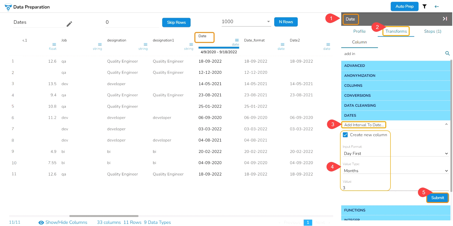
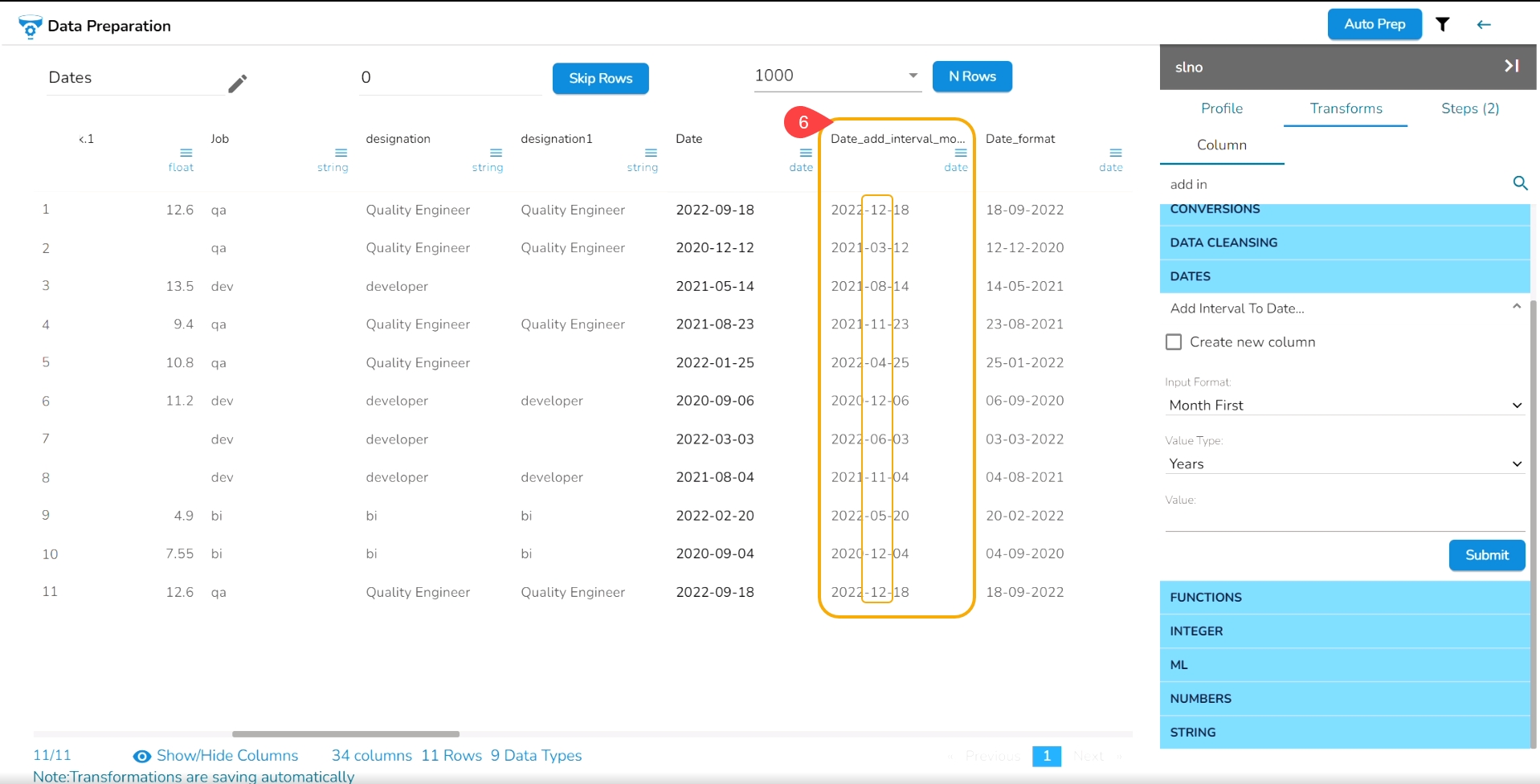
Check out the given walk-through on how to use the Add Interval to Date transform.
Select a column with Date values from the data grid.
Open the Transforms tab.
Select the Add Interval to Date transform from the Dates category.
Enable the Create new column option to create a new column with the transform result.
Input Format: It is used to specify the format of the selected Date column format. It can have values ‘Year first’, ‘Month first’, and ‘Day first.’
Value Type: It specifies the type of duration which acts as the operand for the addition. The value type can be years, months, days, weeks, hours, minutes or milliseconds
Value: The value or the operand that must be added with the selected column
Click the Submit option.
E.g., The Add Interval to Date transform has been applied to the Date column with the selected value of 3 months,
As a result, a new column gets added to the Data Grid reflecting the transformed data as per the set value.
Please Note: The transform supports the datetime column of ‘yyyy-mm-dd’ into the ‘hh:mm:ss’ format.
Converts the DateTime value to the corresponding value of the specified time zone. Input can be a column of Datetime values and it’s assumed to be in the UTC time zone.
Please Note: Inputs with time zone offsets are invalid.
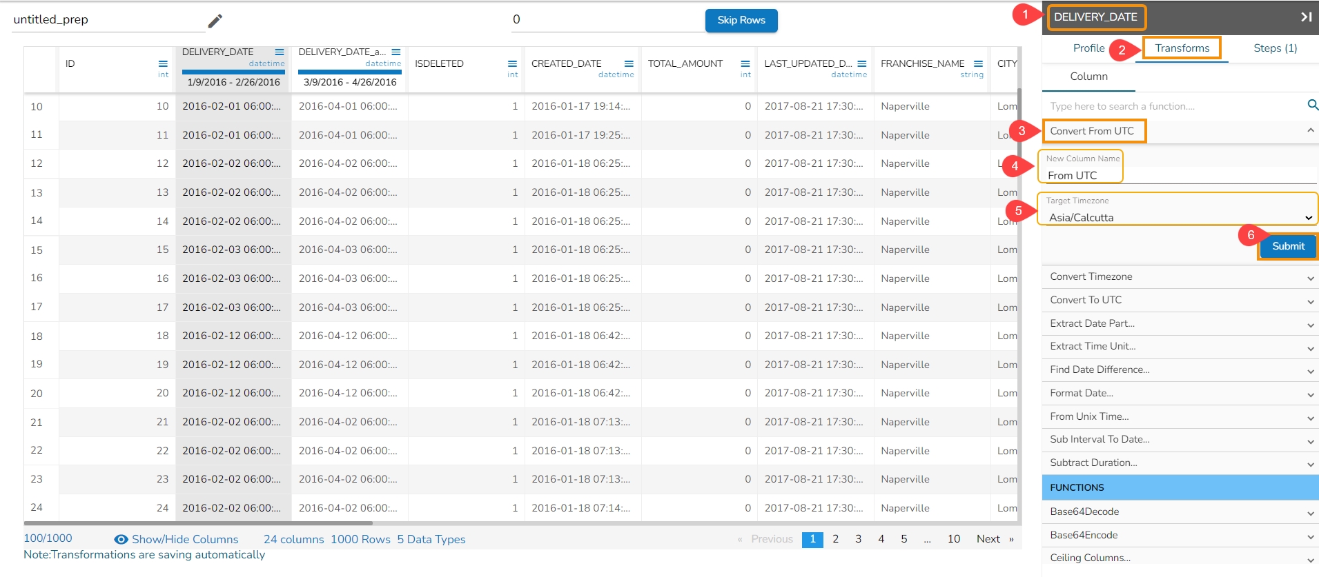
Check out the walk-around on the Convert From UTC transform.
Steps to perform the transformation:
Select a DateTime column from the Dataset.
Navigate to the Transforms tab.
Select the Covert From UTC transform from the Dates category
Pass new column name.
Pass the Target Time zone in which the date to be converted.
Click the Submit option.
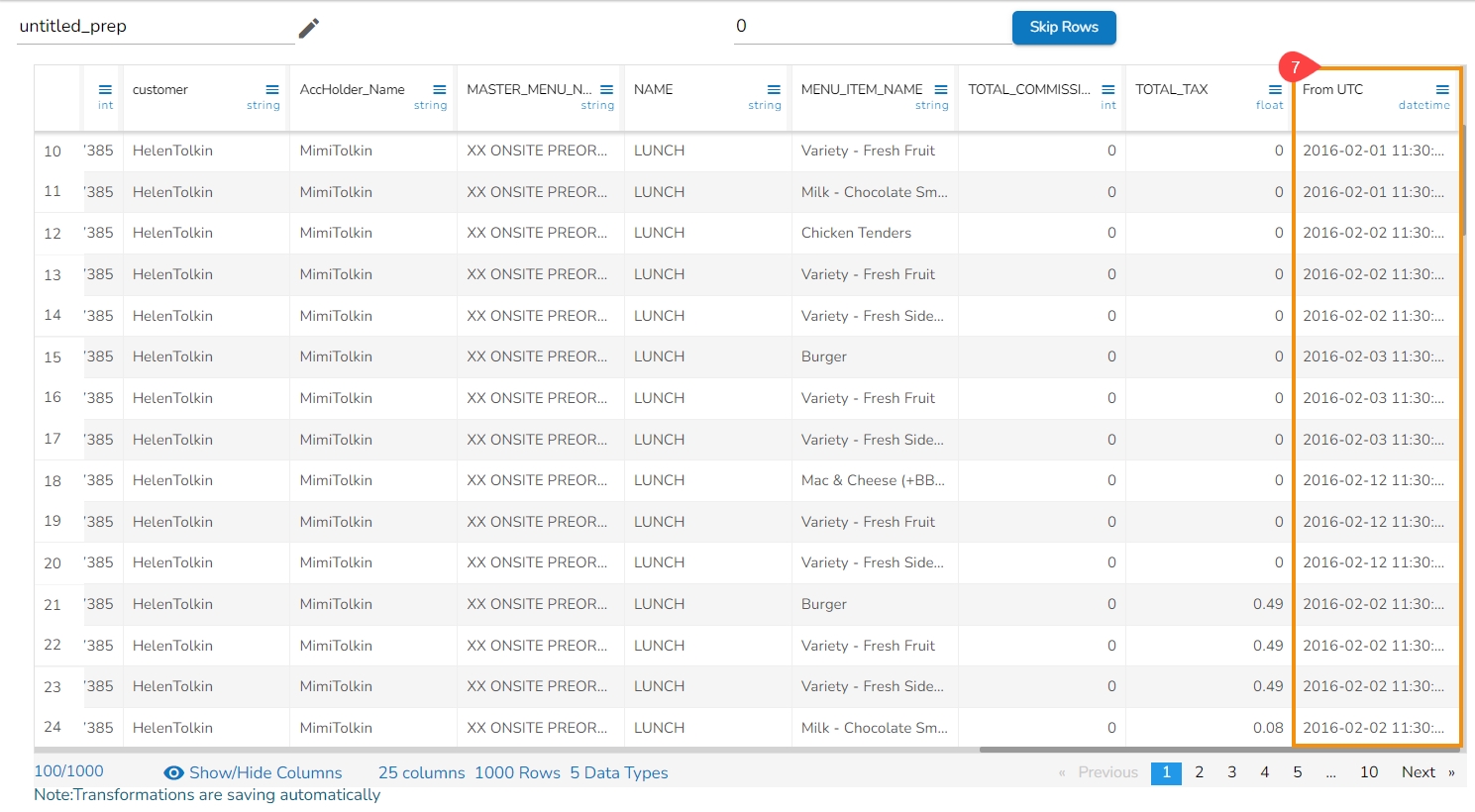
Result will come in a new column with the converted time zone present in it.
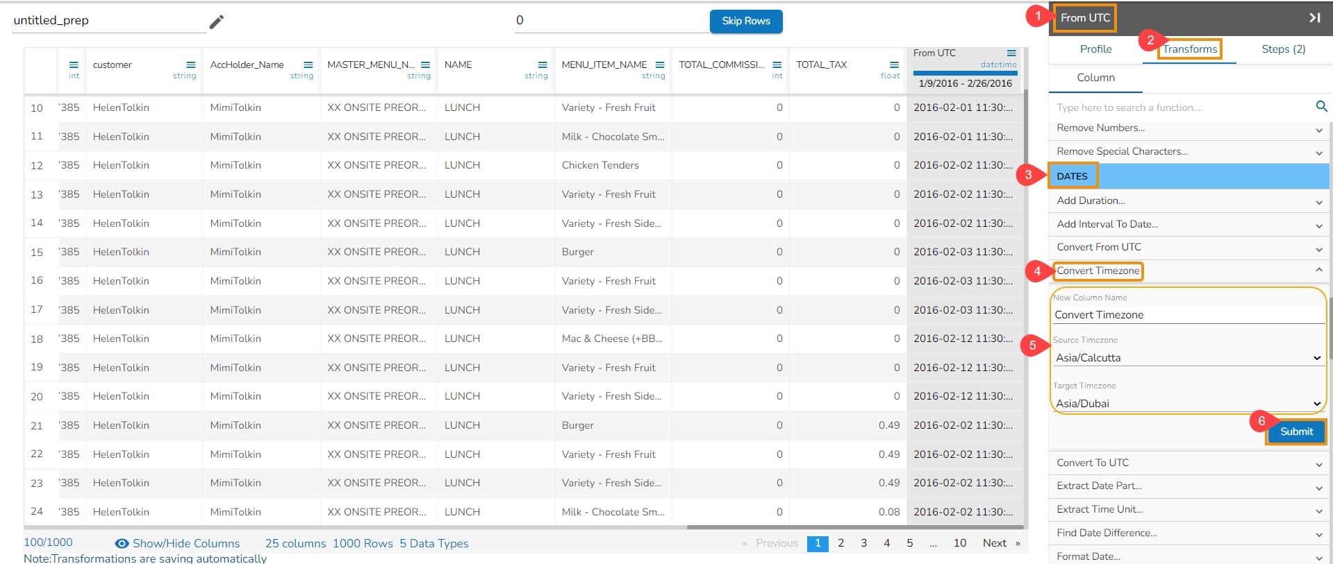
The Convert Timezone transformation converts Datetime value in a specified time zone to corresponding value second specified time zone.
Please Note: Inputs with time zone offsets are invalid.
Steps to perform the transformation:
Select a DateTime column from the Data Grid.
Navigate to the Dates transforms category.
Select the Convert Timezone transform.
Pass new column name.
Pass the Source Time zone for the selected date column.
Pass the Target Time zone in which the date to be converted.
Click the Submit option.
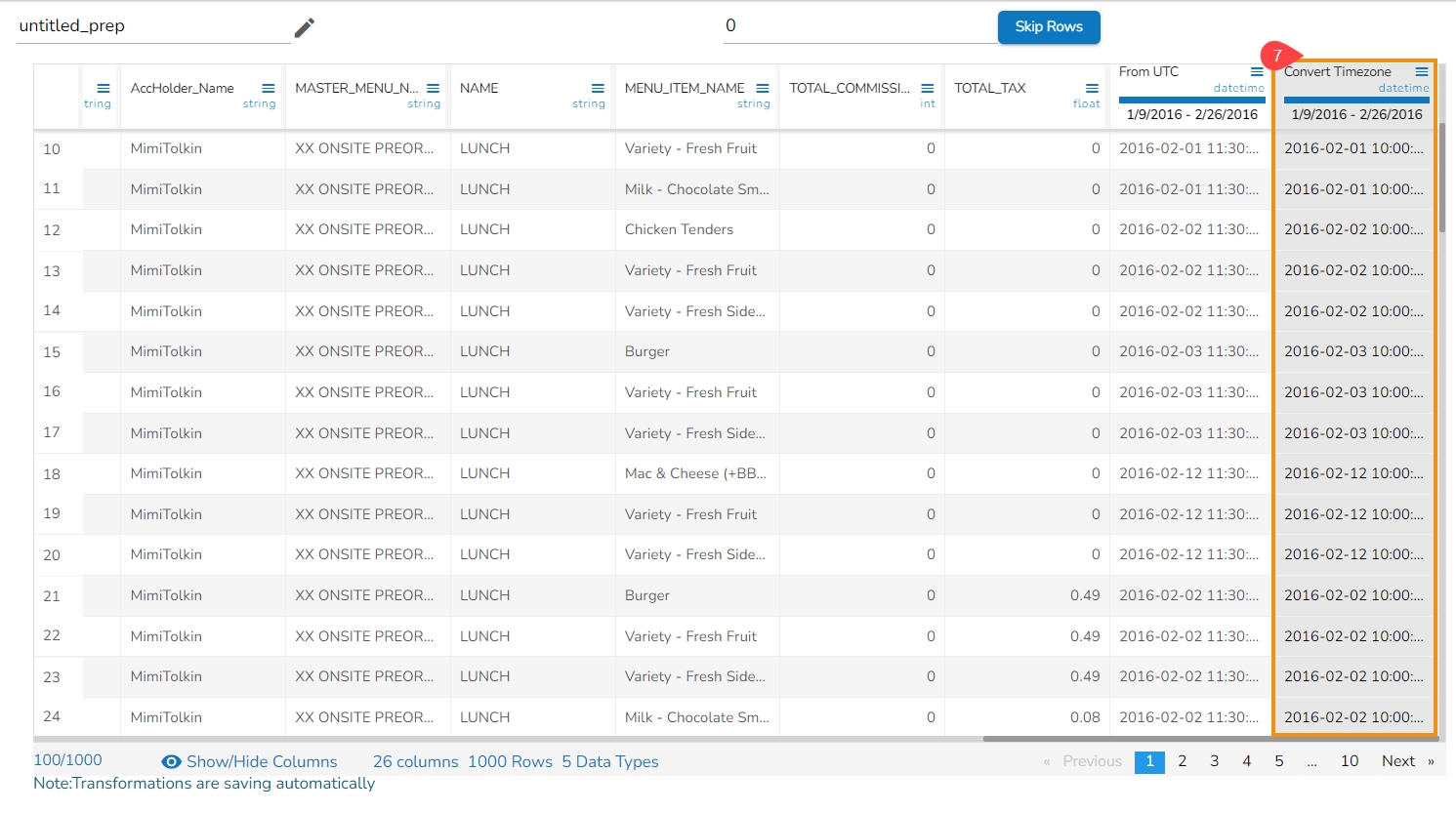
Result will come in a new column with the converted time zone.
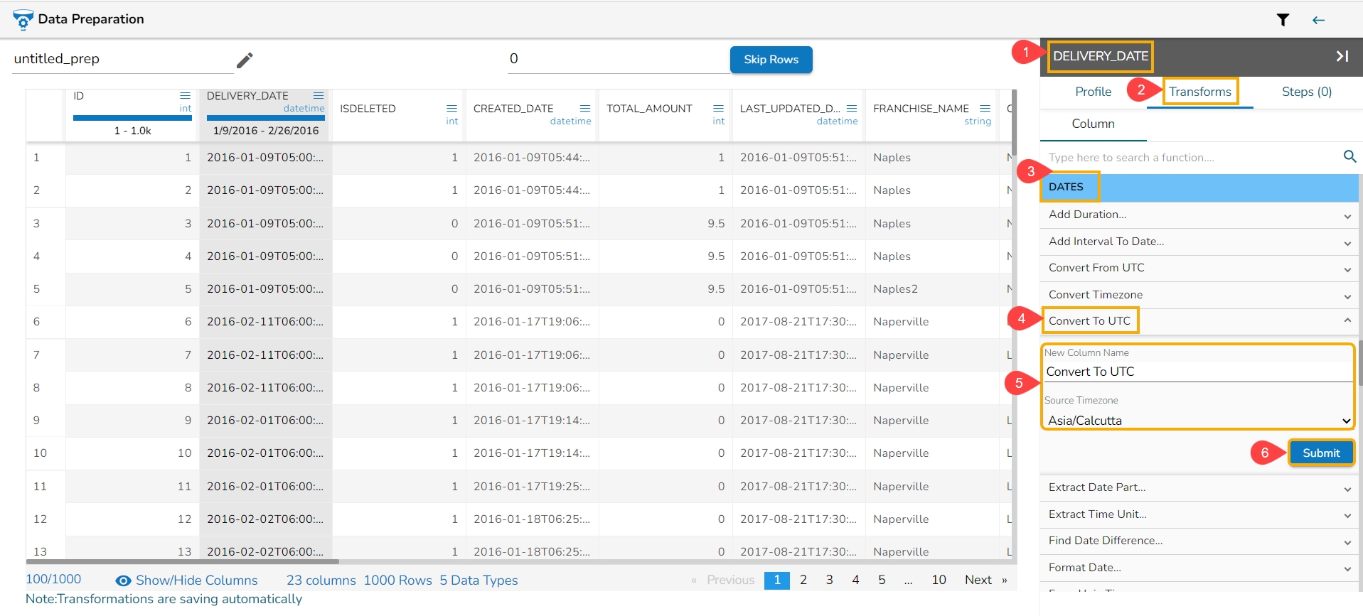
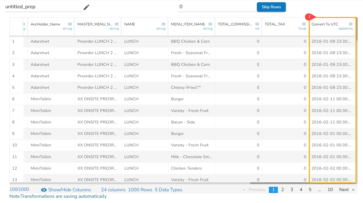
The Convert To UTC transform converts the DateTime value in a specified time zone to the corresponding value in the UTC time zone. Input can be a column of DateTime values.
Check out the given walk-through on how to Convert to UTC.
Please Note: Inputs with time zone offsets are invalid.
Steps to perform the transformation:
Select a DateTime column from the Data Grid.
Open the Transforms tab.
Navigate to the Dates transforms category.
Select the Convert To UTC transform.
Pass new column name.
Pass Source Time zone from which the date is to be converted to UTC.
Click the Submit option.
Result will come in a new column containing the converted UTC format.
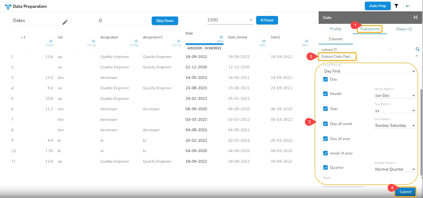
It extracts the date part from a selected column with a date value. The date parts that can be extracted include day, month, year, the day of the week, the day of the year and the week of the year.
Check out the given illustration on how to use the Extract Date Part transform.
Select a Datetime column from the Data Grid.
Open the Transforms tab.
Select the Extract Date Part transform from the Dates transforms category.
Select an Input Format based on the selected column.
Day: It extracts day from a date
Month: It extracts the month from a date/datetime. We can specify the pattern in which the month value has to be returned. Month pattern can be 0-12, Jan - Dec or January - December
Year: It extracts the year from a date. We can specify the pattern in which the year has to be returned. The year pattern can be in the ‘yy’ or ‘yyyy’ format.
Day of Week: It returns the day of the week for the selected date. Day of week pattern can also be specified. The pattern can be 1-7, Sun-Sat or Sunday-Saturday
Day of Year: It returns a number between 1 and 365, which indicates the sequential day number starting with day one on January 1st.
Week of Year: It replaces a number between 1 and 53, which indicates the sequential week number beginning with 1 for the week January 1st falls.
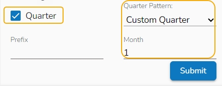
Quarter: It displays the date value based on the quarter, select a quarter pattern using the drop-down option. The supported options are Normal Quarter, Financial Quarter, and Custom Quarter (the user can define the month value for the custom quarter option).
Click the Submit option after selecting all the Date Parts that you wish to extract from the targeted column.
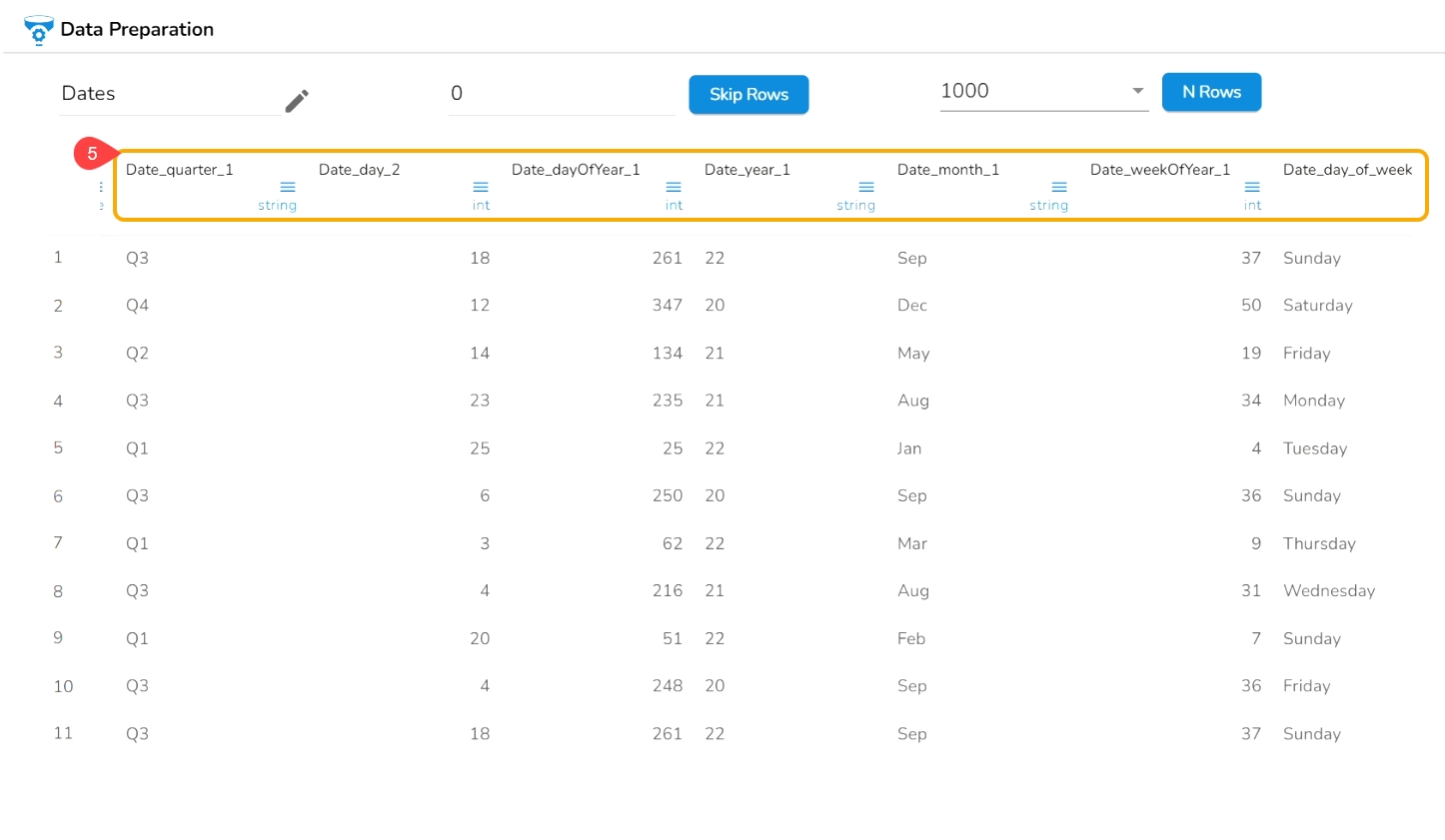
E.g., This transform is applied on the Date column by selecting the Day, Month (Jan-Dec format), Year (in yy pattern), Day of Week (Sunday- Saturday), Day of year, Quarter as a part to be extracted from the selected column values.
As a result, it creates a new columns displaying all the selected transform values.
Please Note: The transform supports Date and DateTimes format (date hh:mm:ss).
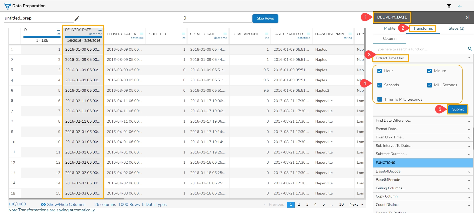
Extract the time units from a selected column with a time value. The time units that get extracted include hours, minutes, seconds, milliseconds, and time to milliseconds.
Select a Datetime column from the Data Grid.
Open the Transforms tab.
Select the Extract Time Unit transform from the Dates transforms category.
Hours: Extracts hours from a time
Minutes: Extracts minutes from a time
Seconds: Extracts seconds from a time
Milliseconds: Extracts milliseconds from a time
Time to Milliseconds: Converts the time given to milliseconds
Click the Submit option.
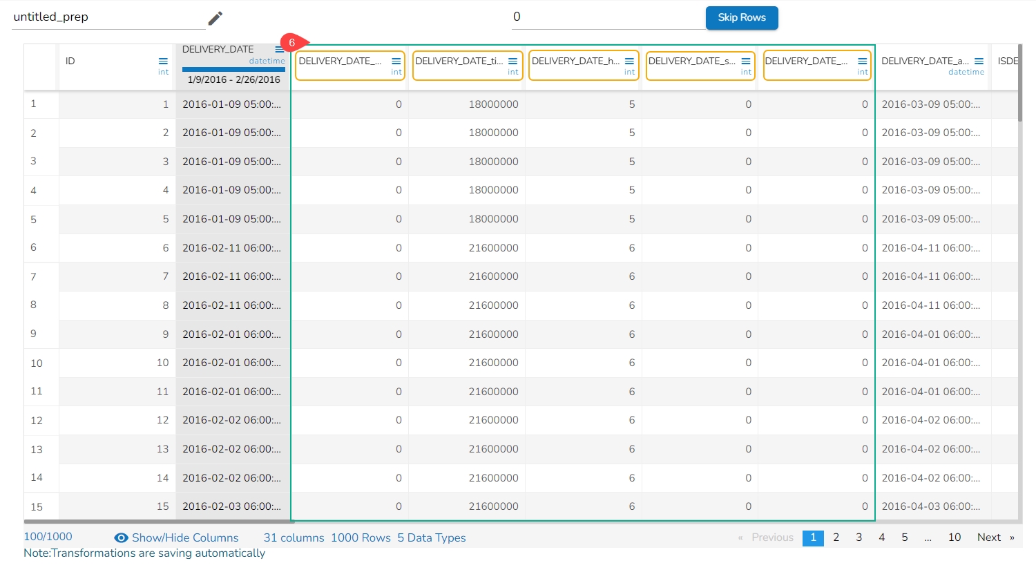
The Extract Time Unit transform is applied to the DELIVERY_DATE column selecting all the available format types:
As a result, the time gets extracted in the set time units and no. of columns get added based on the selected time unit options. E.g., In this case, 5 new columns get added to the Data Grid displaying the extracted time values.
Please Note: The transform supports time format like- hh:mm:ss:mmm, hh:mm:ss, hh:mm
The transform finds the difference between two date values. It can either subtract the selected column with a date value or date from another column. The transformed value can replace the existing column value or can be added as a new column.
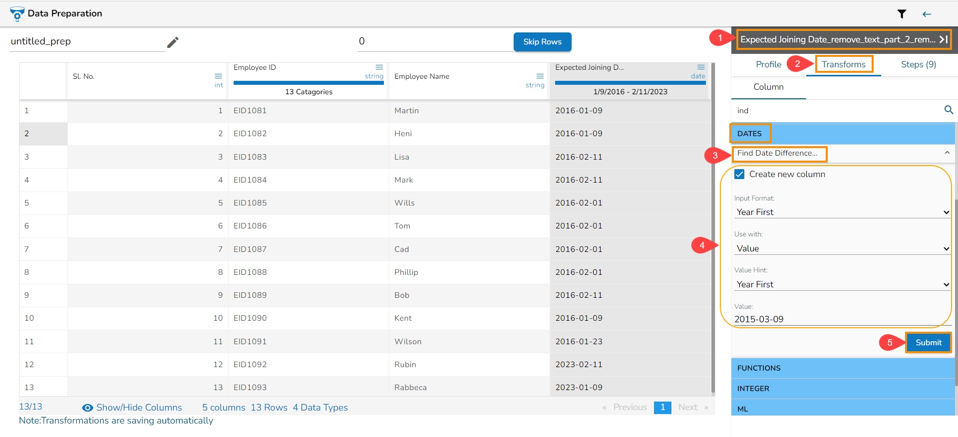
Select a Date column from the Data Grid.
Open the Transforms tab.
Select the Find Date Difference transform from the Dates transforms category.
Enable the Create new column option to create a new column with the transformed data.
Input Format: Specifies the format of the given date column.
Use with: Specify whether to fill with a value or another column value.
Value Hint: Specify format of value from which you want to find the difference.
Value: Pass the date value from where you want to find the date difference.
Click the Submit option.
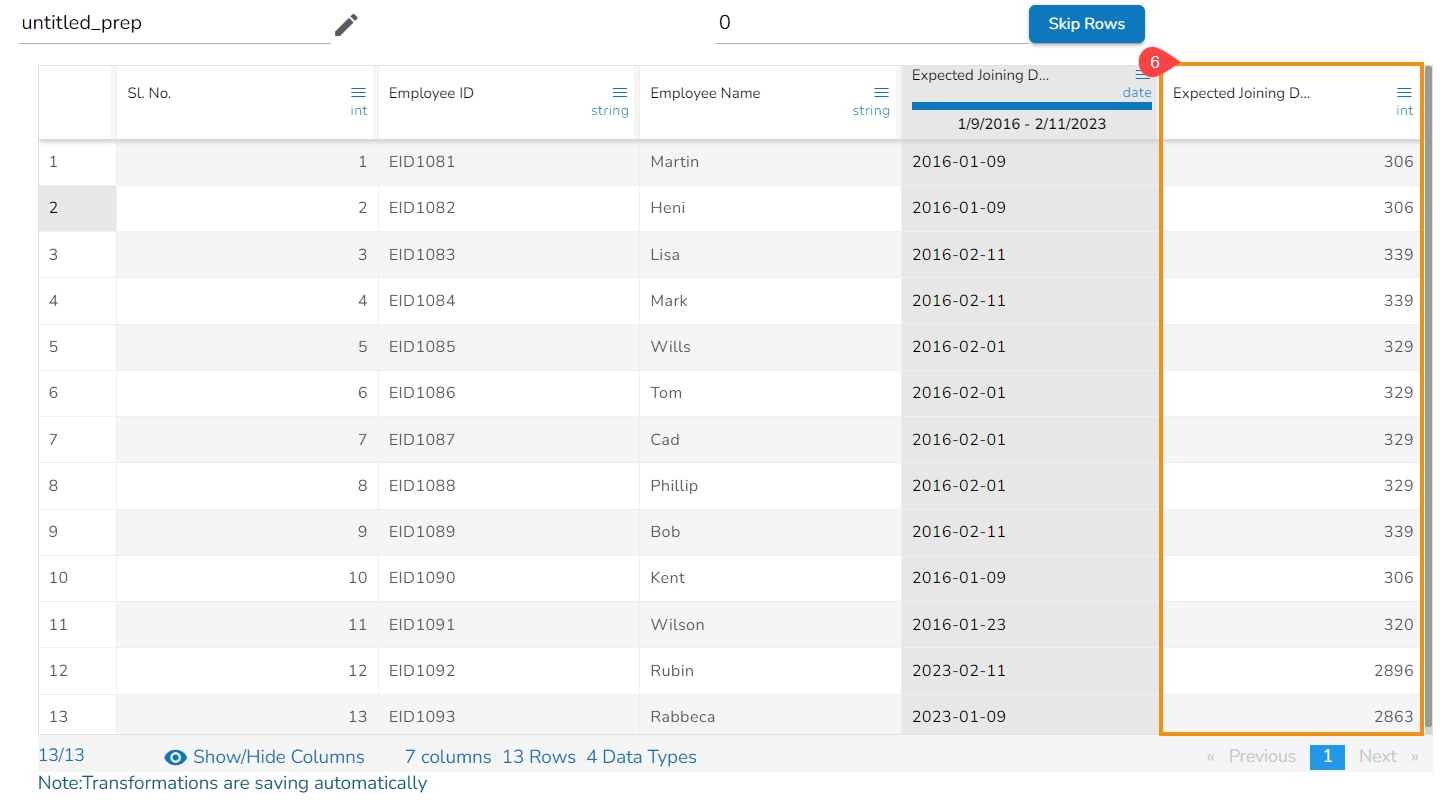
In this case, the Find Date Duration transform has been used with the value 2015-03-09.
As a result, a new column gets created with the set Date Duration value.
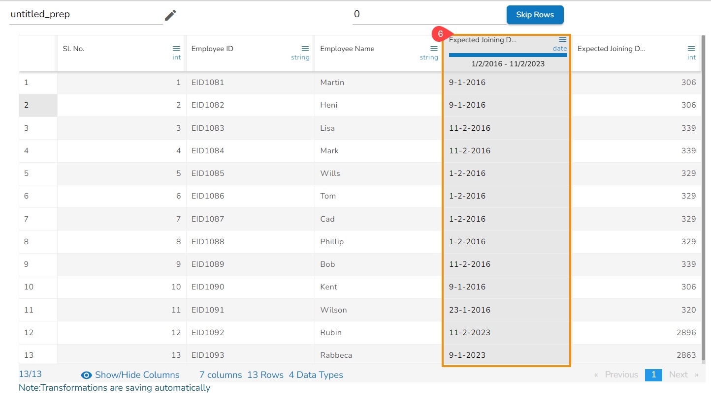
The users can change the format of a date column by using this transform.
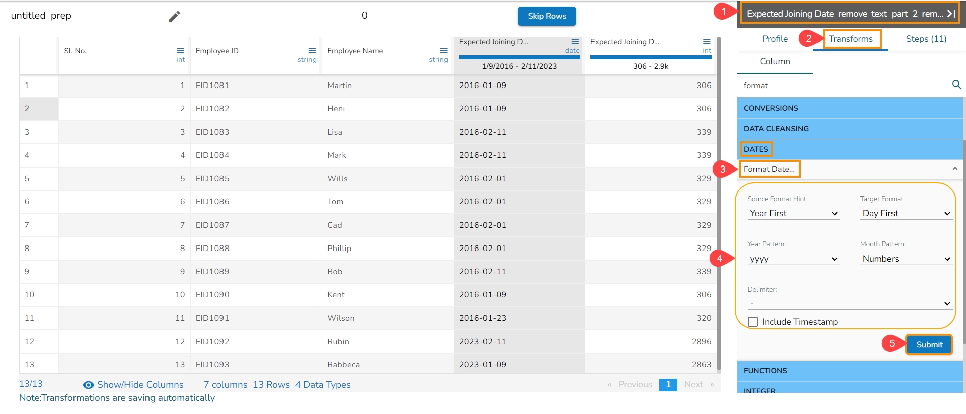
Select a Date column from the Data Grid.
Open the Transforms tab.
Select the Format Date transform from the Dates transforms category.
Source Format Hint: Specifies the current format of the date column.
Target Format: Specifies what we want first (Year, Month, Day) in our output format of the date column.
Year Pattern: Specifies the format of the year (yyyy or yy) in the output date column.
Month Pattern: It specifies the format of the month (number, Jan-Dec, January-December) in the output date column.
Delimiter: Specifies Delimiter (like- slash, a hyphen, comma, full stop, space) for the output date column.
Include Timestamp: It adds a timestamp to the current date format if enabled with a tick mark.
Click the Submit option.
As a result, it displays the values of the selected column as per the set transform format of Date:
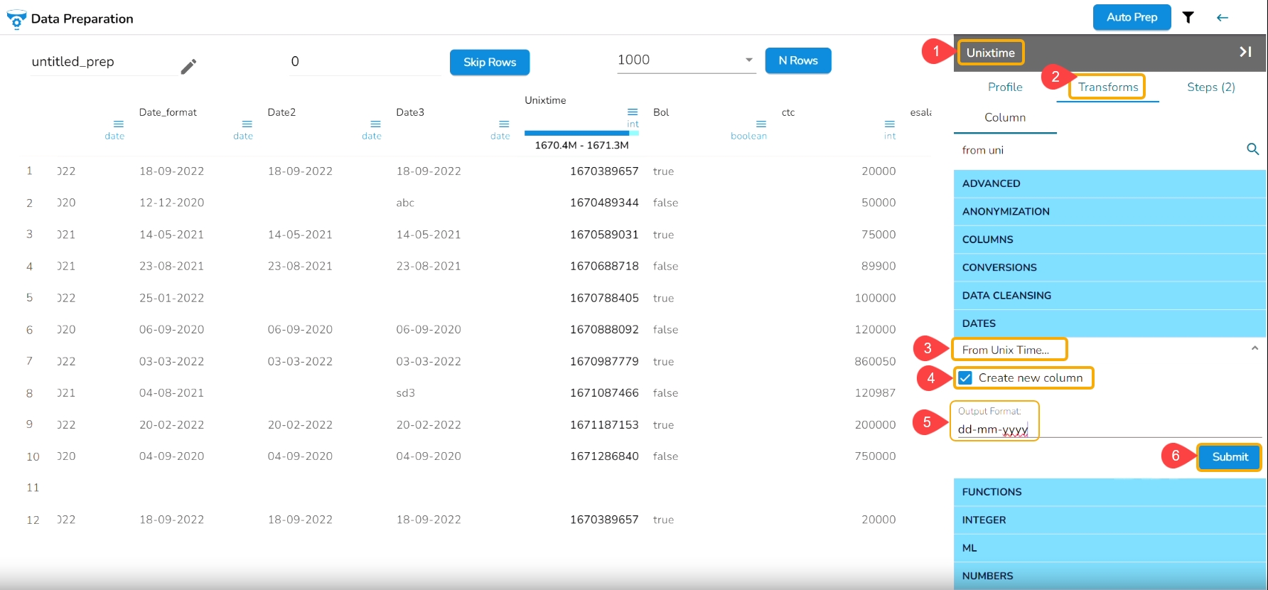
The From Unix Time transform converts the Unix time into a specified format. The From Unix Time transform has been applied on the Date column that contains the values in the Unix format.
Check out the given illustration on how to user From Unix Time transform.
Select a Date column from the Data Grid that contains data in the Unix time.
Open the Transforms tab.
Select the From Unix Time transform from the Dates transforms category.
Enable the Create new column option to create a new column with the transformed data values.
Provide the Output Format in which you want to get the result data.
Click the Submit option.
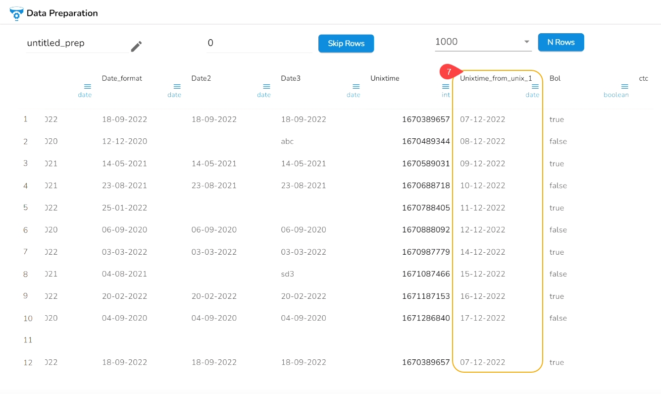
As a result, a new column gets added to the Data Grid in the set Date format with the converted Unix values:
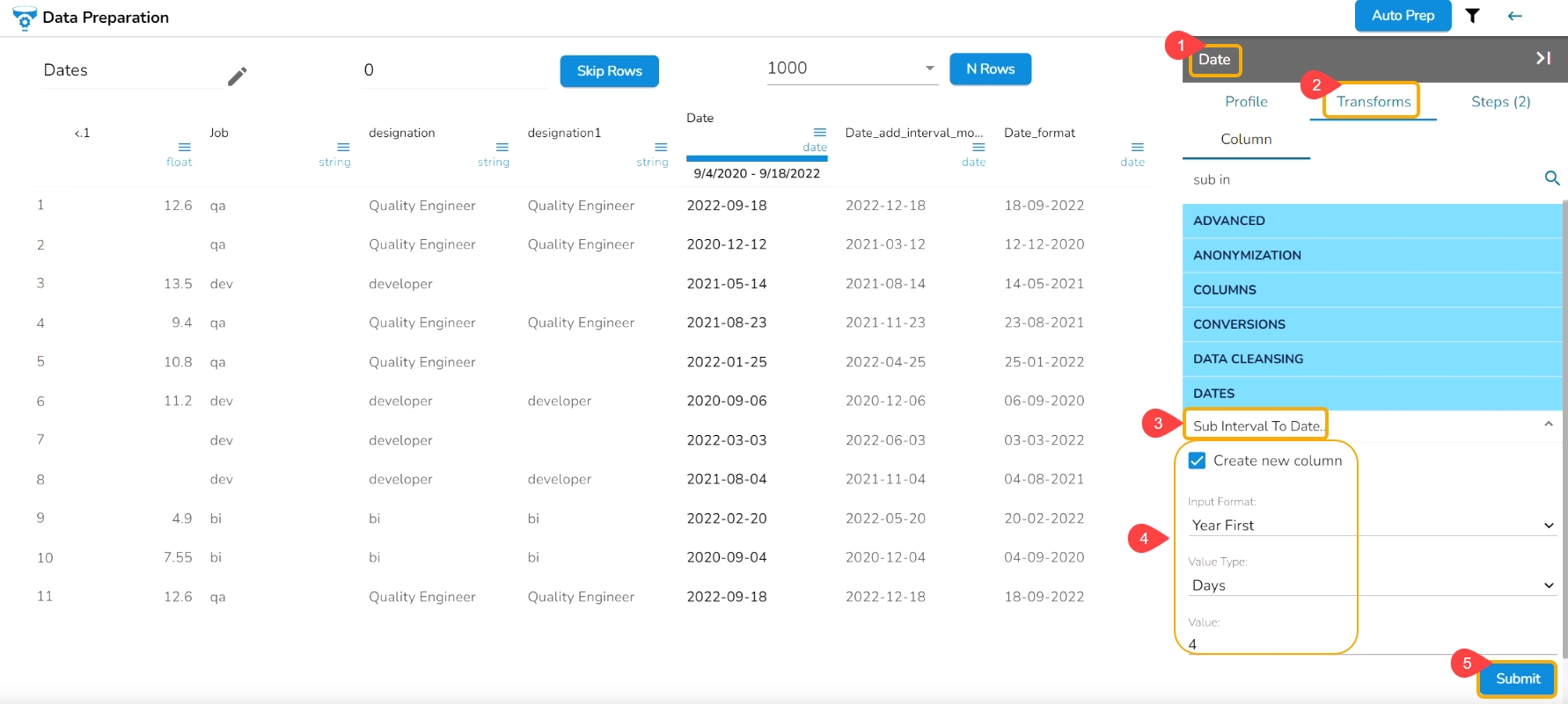
The Sub Interval to Date transform subtracts specified value(interval) from the given date column. The transformed value can replace the existing column value or can be added as a new column.
Check out the given illustration on how to use Sub Interval to Date.
Select a Date column from the Data Grid.
Open the Transforms tab.
Select the Sub Interval to Date transform from the Dates transforms category.
Provide the following information to apply the transform:
Enable the Crate new column option to create a new column with the transformed values.
Input Format: Format of date column(given) should be specified here.
Value Type: It specifies what we want to subtract like years, months, days, weeks, etc.
Value: It specifies how many years/months/days (value type) we want to subtract.
Click the Submit option.
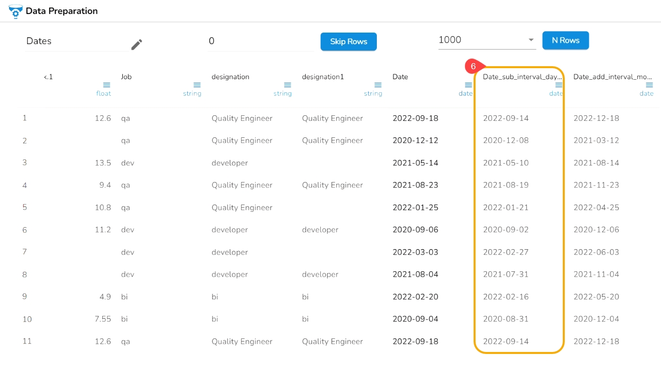
E.g., The Sub Interval to Date transform is applied on the Date column with the 4 days as value to get Sub Interval to the given date.
As a result, a new column gets created with the set sub interval values:
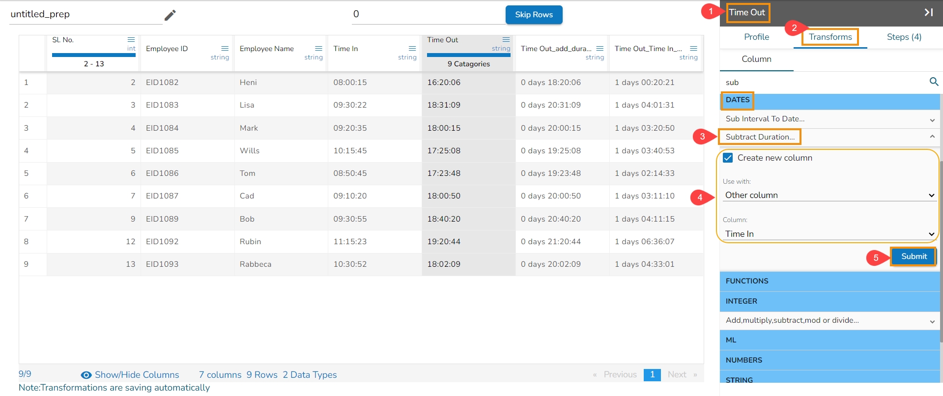
The transform ‘Subtract Duration’ deducts the time values in two ways. It can either subtract the selected column with a time value or time from another column. The transform supports subtracting time into ‘hh:mm:ss.mmm’,‘ hh:mm:ss’, and 'hh:mm’ formats. The transformed value can replace the existing column value or can be added as a new column.
Select a column with the time values from the dataset.
Navigate to the Transforms tab.
Select the Subtract Duration transform from the Dates category.
Enable the Create new column option, if you wish to create a new column with the result data.
Use with: Specify whether to fill with a value or another column value
Column/ Value: The value with which the column must be subtracted, or the column with which the selected column value must be subtracted.
Click the Submit option.
The result will get displayed based on your Use with selection as described below:
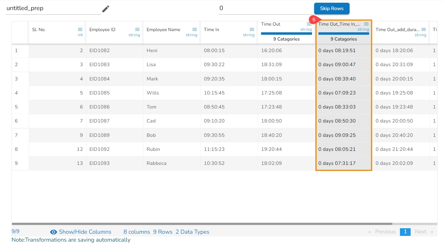
The Subtract Duration transform has been applied to the Time Out column, the selected other column is Time In,
As a result, a new column gets added to the Data Grid with the subtracted duration out of the selected columns:
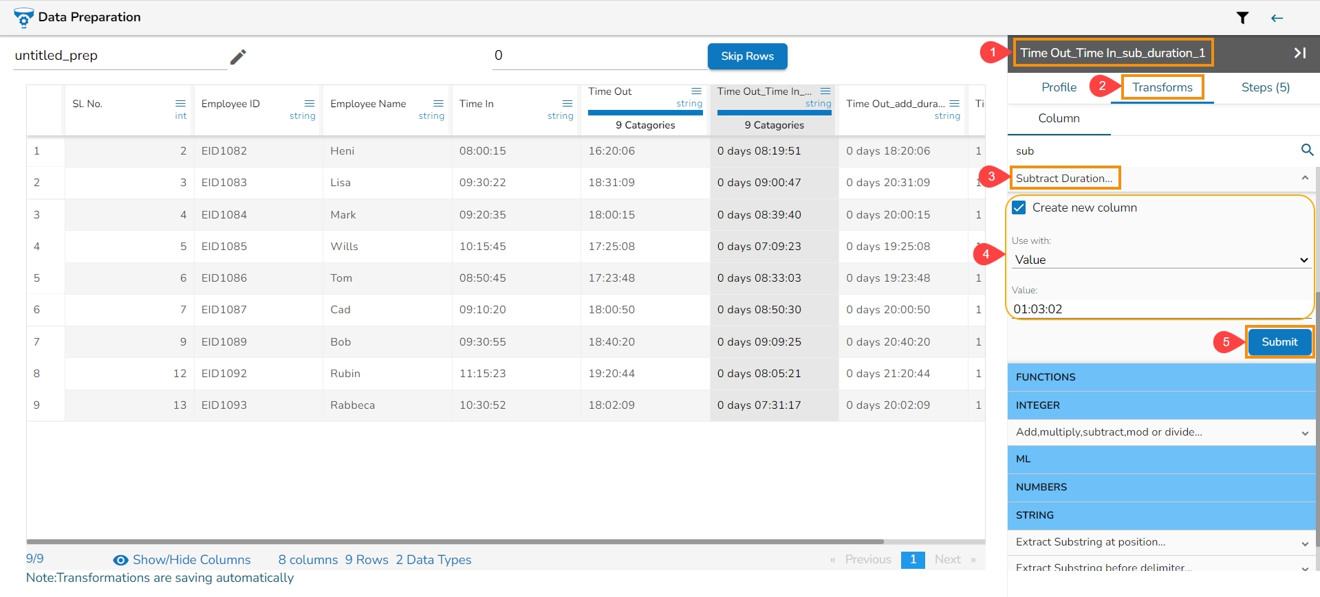
The Subtract Duration transform has been applied to the Time Out_Time In_sub_duration_1, the selected value is 01:03:02,
As a result, a new column gets added to the Data Grid with the remaining values after subtracting the set values from the targeted column:
Pay Attention: The Delete Columns Except transform is renamed as Keep Column.
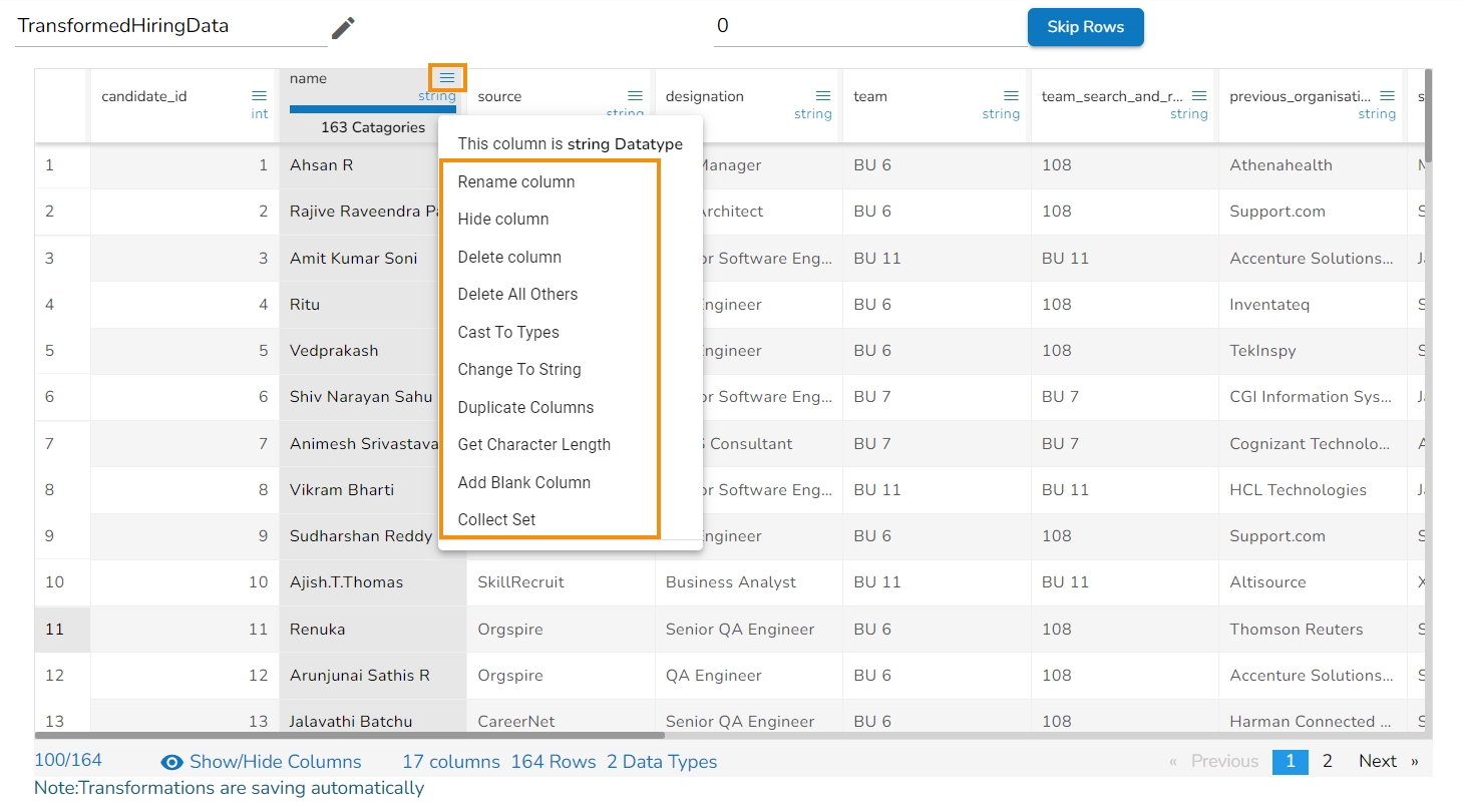
Some of the Column transforms can be accessed by using the Menu icon provided for each column in the Data Grid display of the dataset.
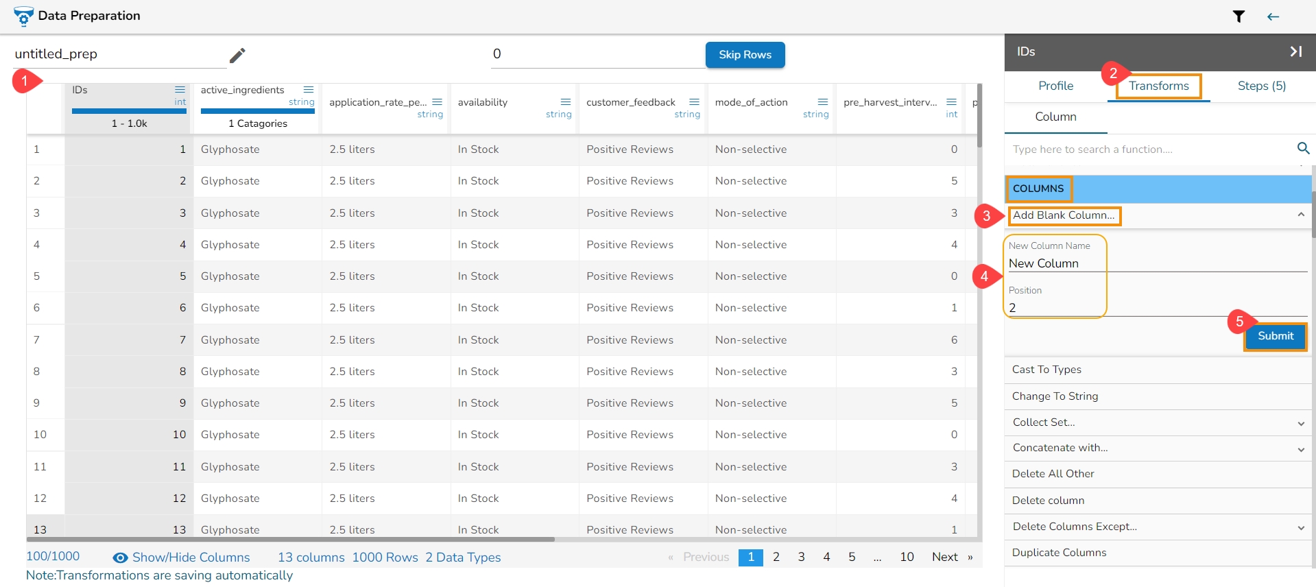
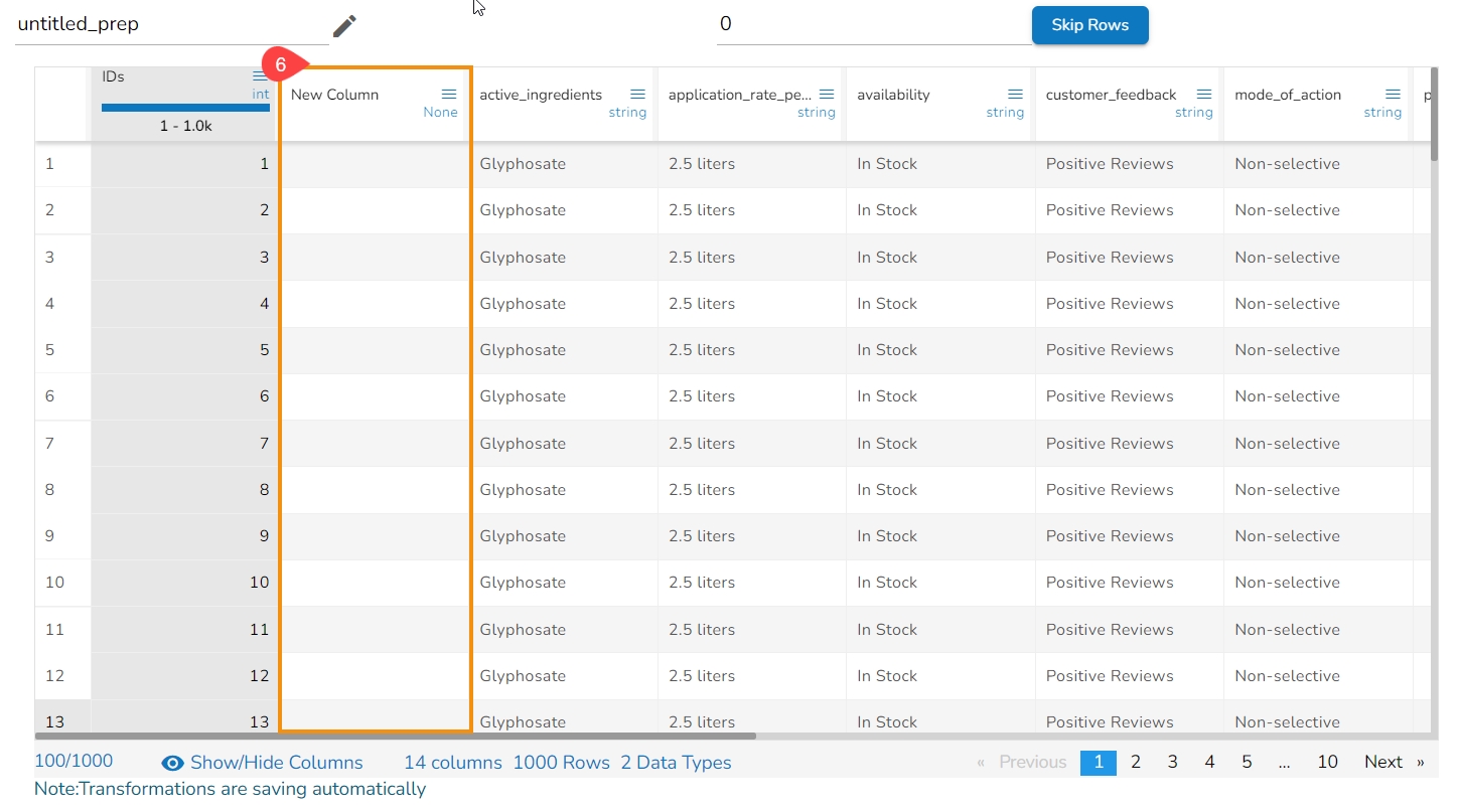
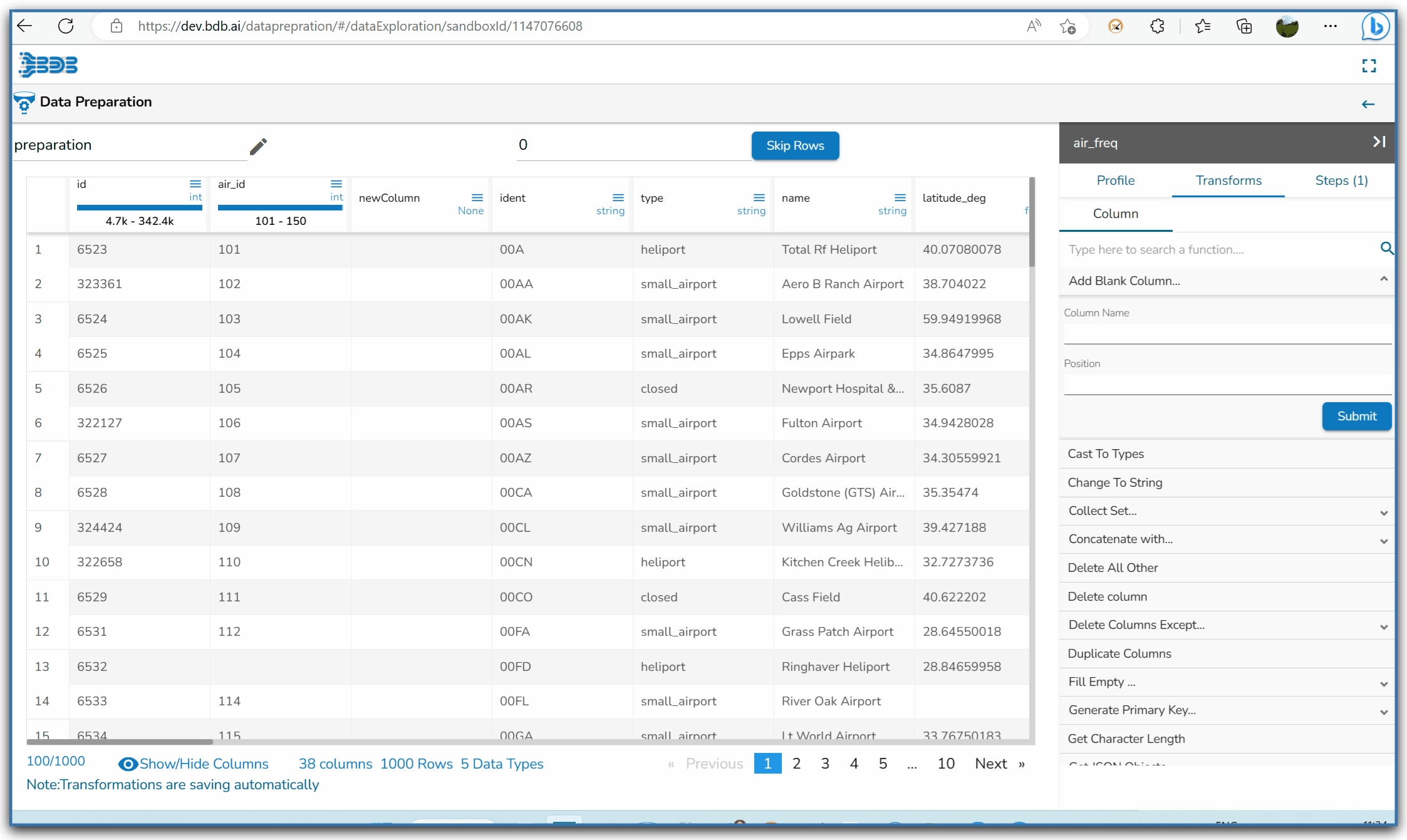
This transform will create a new blank column in the selected data set. The datatype for the newly added blank column will be as None.
Navigate to the Data Preparation page displaying data grid.
Open the Transforms tab.
Select the Add Blank Column transform from the Column transforms type.
Provide the required details:
New Column Name
Position (of the blank column)
Click the Submit option.
The empty column gets added in the dataset (at the selected position with the provided name).
Please Note:
The user can update values in this column by using the transforms like Fill empty, Search & Replace.
The Add Blank Column transform can also be accessed by using the menu icon provided for the each column in the Data Grid display of the dataset.
The Array to Column data transform returns the array data separated in multiple columns.
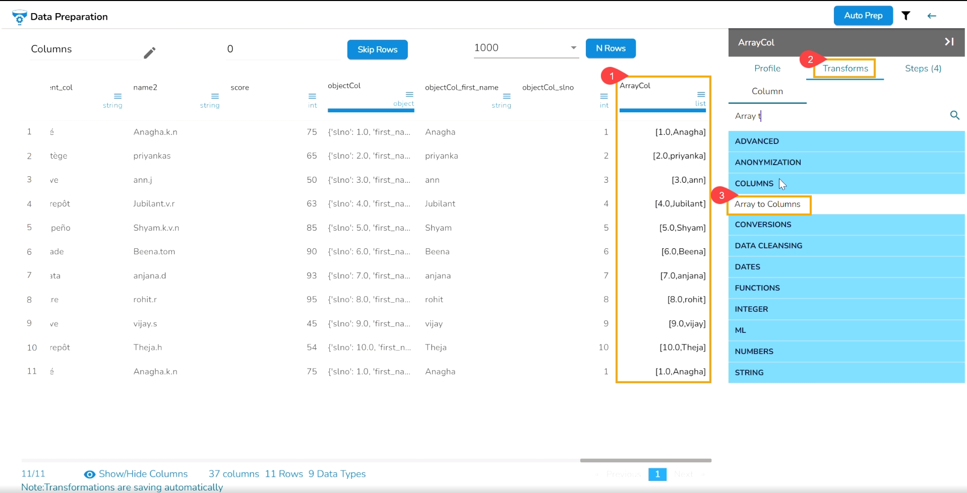
Check out the given walk-through on how to use the Array to Column transform.
Select a column with array data from the dataset within the Data Preparation framework.
Open the Transforms tab.
Select the Array to Columns transform from the COLUMNS category.
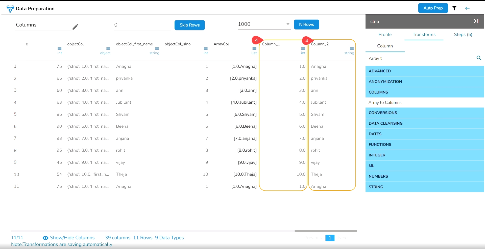
As a result the array data will be separated in the multiple columns (based on the available data the no. of the columns will be added).
Please Note:
Based on the maximum count of values given in the array format the no. of result columns will be added.
E.g., The above-given example contains two data values in the array format, so there are 2 columns created as the result.
The names of the result columns will be auto-generated. E.g., Column_1, Column_2
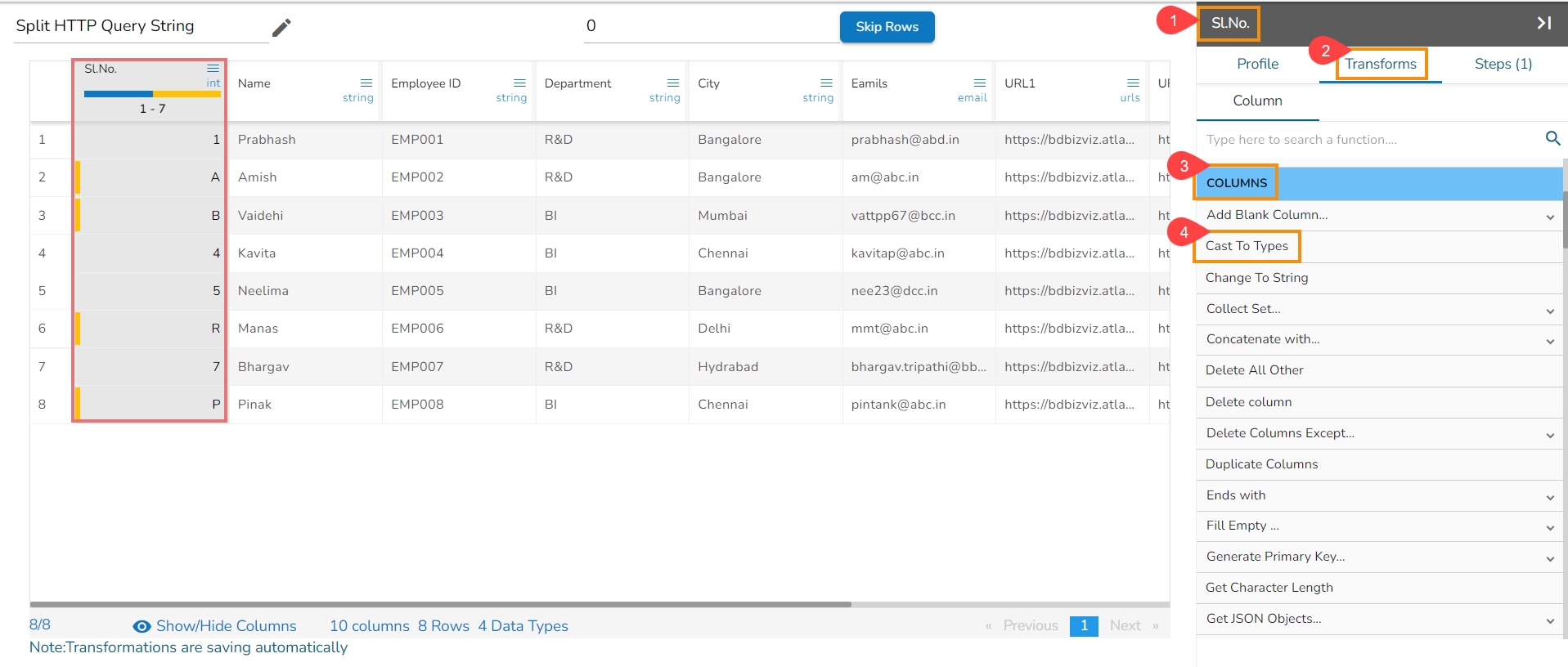
It is a table-based operation. The profiling of a column is done based on the data type present in the majority.
Let’s say in column A; there are four integer values and one string value, then the data type of the column gets profiled as the integer despite one string value present in it.
The Cast to Types transform removes the value with the invalid data type. In this case, it converts data with a string data type to the null value.
Navigate to the Data Preparation displaying data grid.
Select the field that has some invalid values in string data type.
Open the Transforms tab.
Click on the Cast to Types transform from the COLUMNS category of transforms.
The invalid values from the selected column gets removed.
Please Note:
There is a possibility of some data loss while applying this transform to any dataset.
The Cast to Types transform can also be accessed by using the menu icon provided for the each column in the Data Grid display of the dataset.
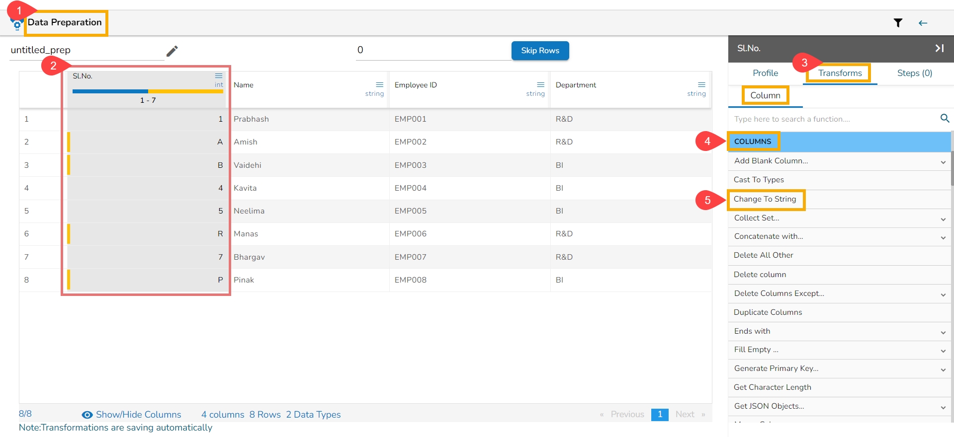
This transformation helps to change the datatype of a selected column into a String.
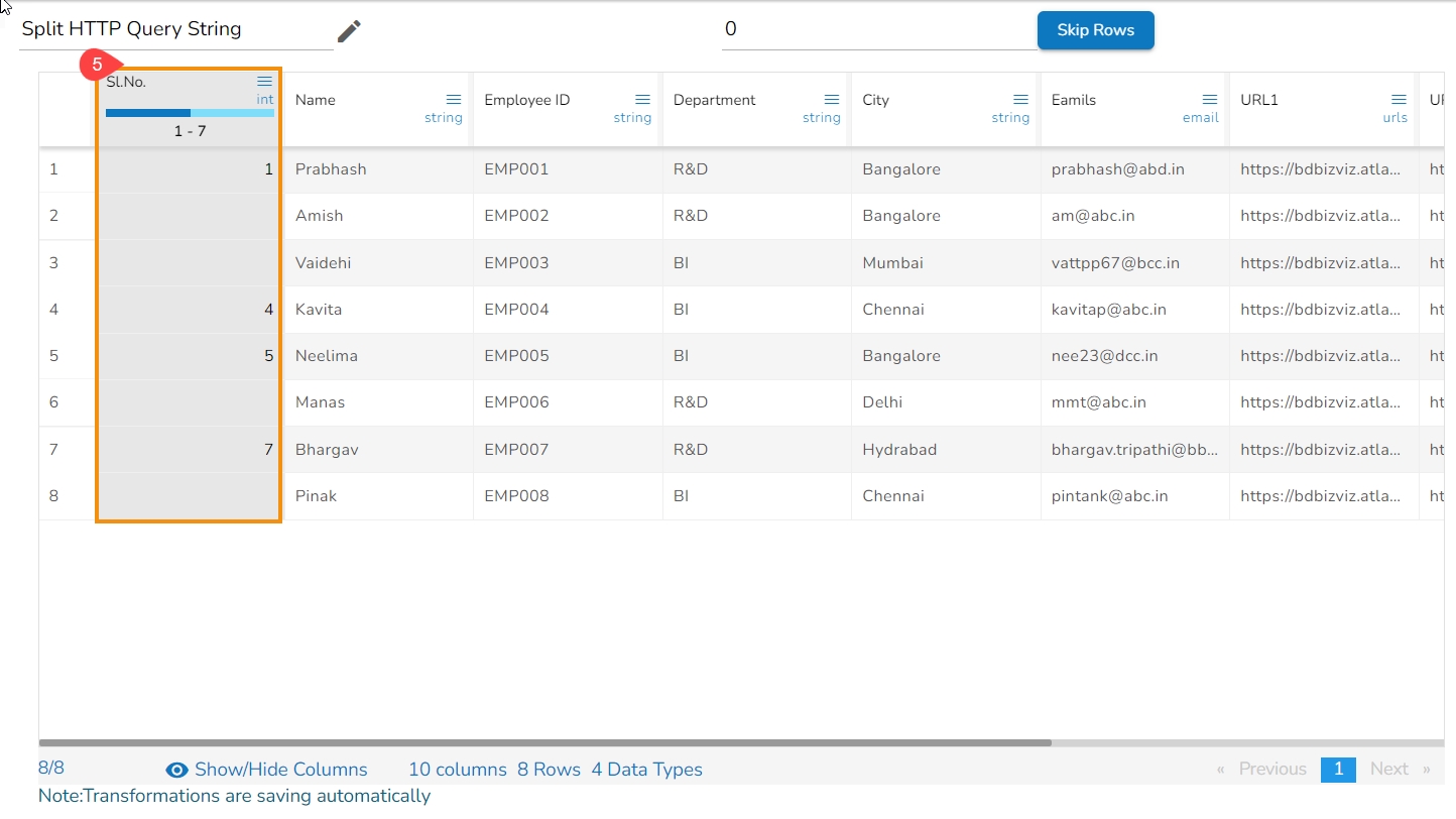
Navigate to the Data Preparation displaying data grid.
Select the field that has some invalid values in string data type.
Open the Transform tab.
Navigate to the Columns type of transforms.
Click on the Change to String transform.
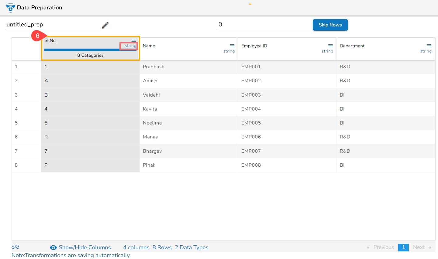
The data type of the selected column gets changed into String.
Please Note:
It will not support Date columns to change into String.
The Change To String transform can also be accessed by using the menu icon provided for the each column in the Data Grid display of the dataset.
The Collect Set transform generates the list of all the unique values of the column based on the selected column. It performs group concatenation.
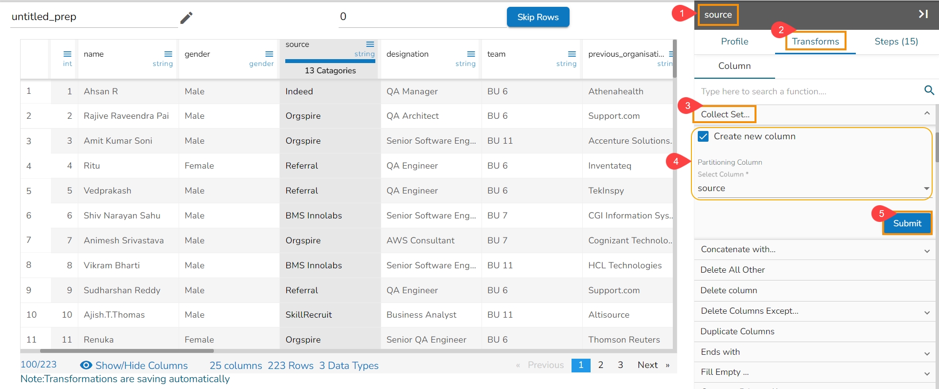
Select a column from the dataset within the Data Preparation framework.
Navigate to the Transforms tab.
Select the Collect Set transform from the COLUMNS transforms.
Enable the Create new column to create a new column with the result of the transformation.
Select a Partitioning column using the drop-down menu. E.g., The selected Column is source.
Click the Submit option.
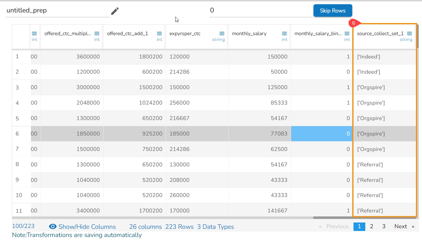
It generates a list of all unique values under the source_collect_set_1 as displayed in the below image:
Please Note: The Collect Set Transform option can also be accessed from menu icon provided for each column in the Data Grid display of the dataset.
Concatenating arrays means combining two or more arrays to create a single, larger array.
Check out the given video on Concatenate Array transform.
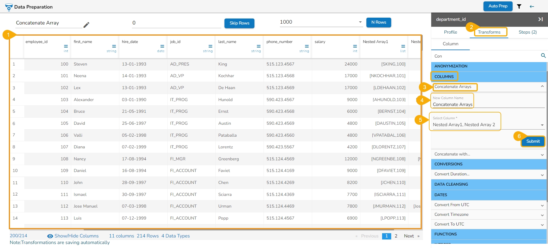
Open a dataset within the Data Preparation framework.
Open the Transforms tab.
Navigate to the Concatenate Arrays transform from the COLUMNS category.
Provide a name for the New Column Name that will get added with the output.
Select the columns with array (list datatype) data. using the Select Column drop-down menu.
Click the Submit option.
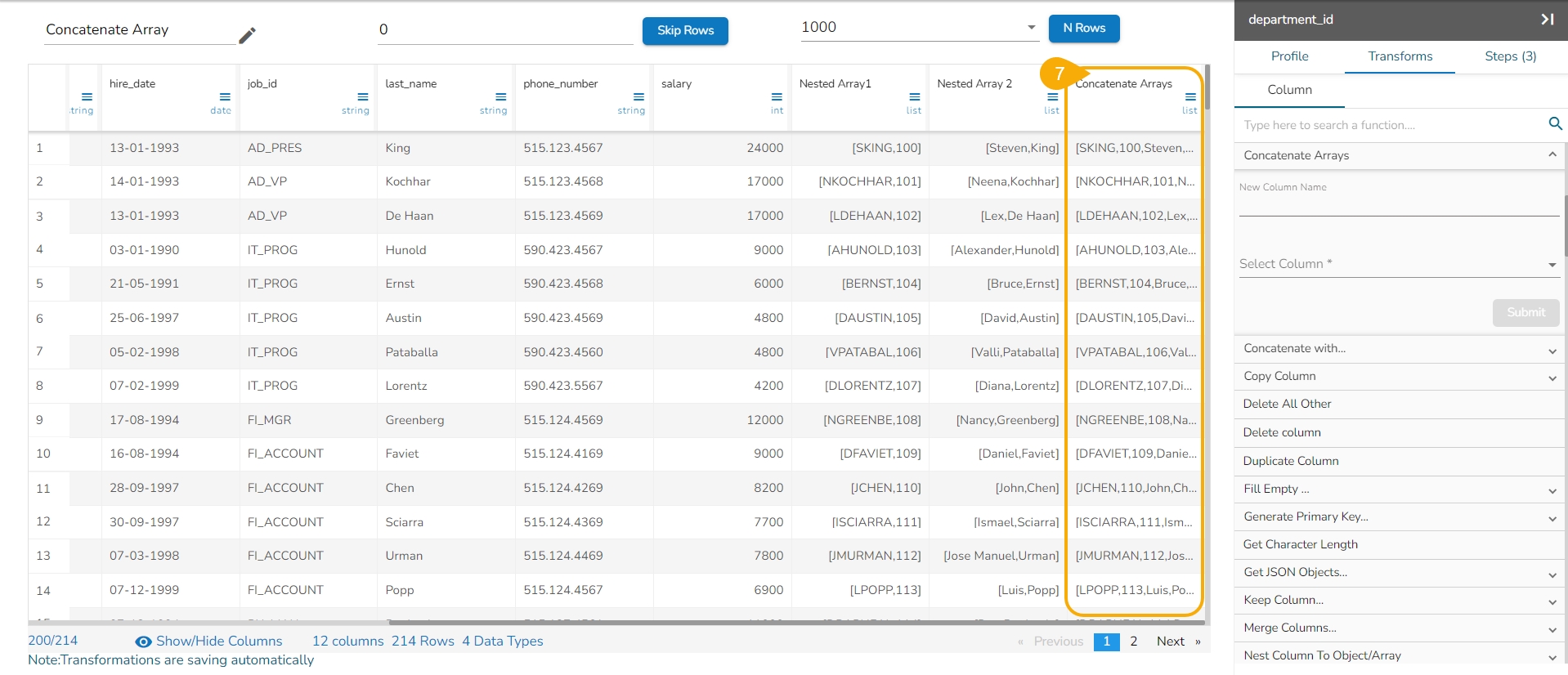
The result will appear displaying the concatenated arrays in a new column with the same name that has been provided by the user.
E.g.,
Please Note: The Concatenate Arrays works only upon the List data type columns.
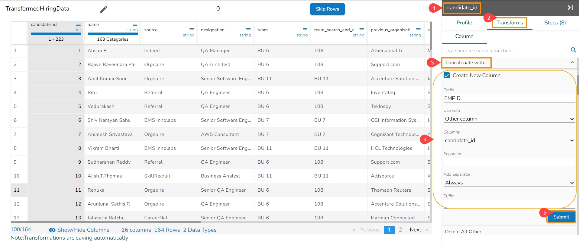
The users can concatenate a column value with some other column or with some prefix/suffix. To perform the transform, select the column to which data must be concatenated and select the Concatenate with transform. The available options are:
Select a column from the Data set.
Open the Transforms tab.
Select the Concatenate with transform from the COLUMNS category.
Prefix: Specify the value to be prefixed to the selected column value
Use with:
Select the Value to add a Prefix/Suffix
Select the Other column to concatenate two columns
Separator: Provide a separator to separate the targeted prefix or suffix from the original column values.
Add Separator: Select an option either Always or Both values not empty when you want to add separator.
Suffix: Provide a value to be used as a suffix to the selected column value.
Click the Submit option.
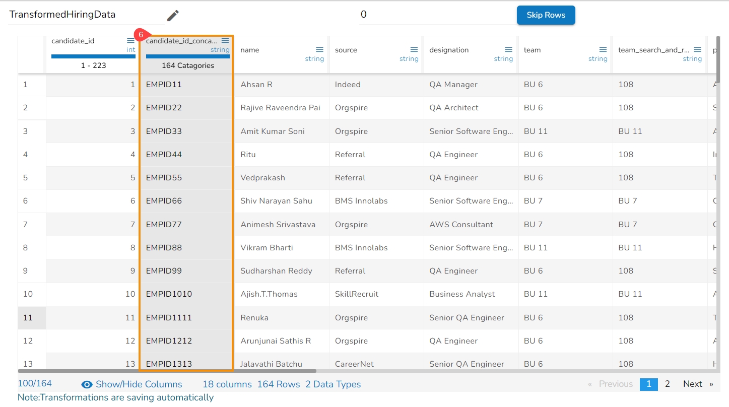
A new column gets added based on the configured details.
Please Note: The users must select the Use with Other Column option to concatenate a value with another column and select the Use with Value option to add prefix/suffix.
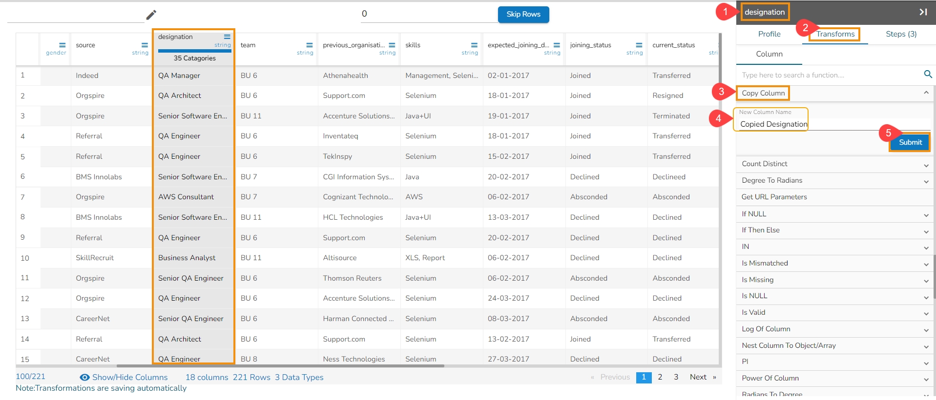
This transformation helps to duplicate the content of a column into another one.
Steps to perform the transformation:
Select a source column from the dataset.
Open the Transforms tab.
Select the Copy Column transform from the FUNCTIONS tab.
Provide name for the new column.
Click the Submit option.
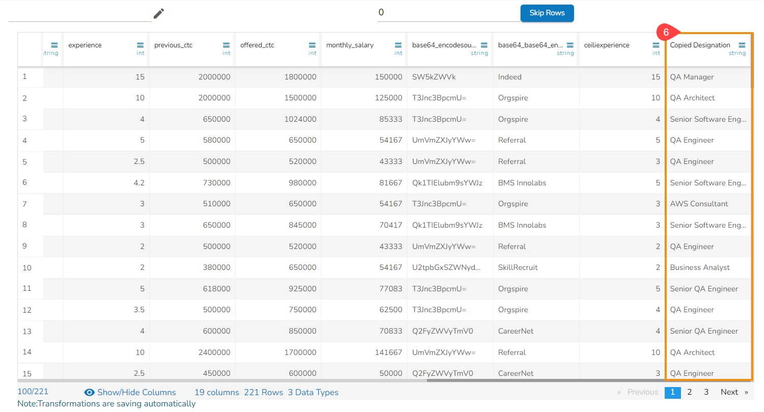
Result will get displayed where the content is duplicated into a new one with a new column name.
Check out the given walk-through on how to use the Copy Column transform.
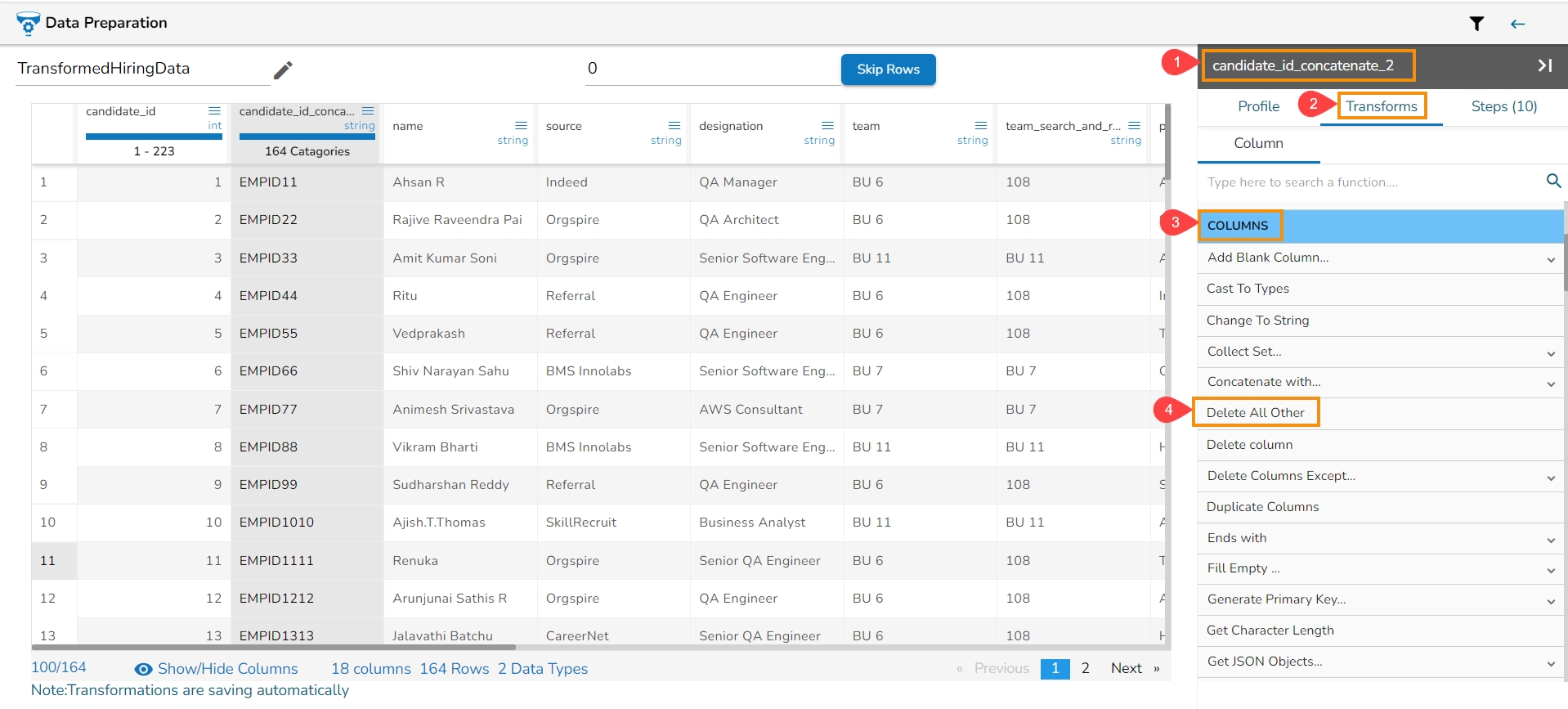
The Delete All Other transform is used to delete all other columns than the selected column.
Select a column from the Data Grid.
Open the Transforms tab.
Open the COLUMNS transform category.
Select the Delete All Other transform.
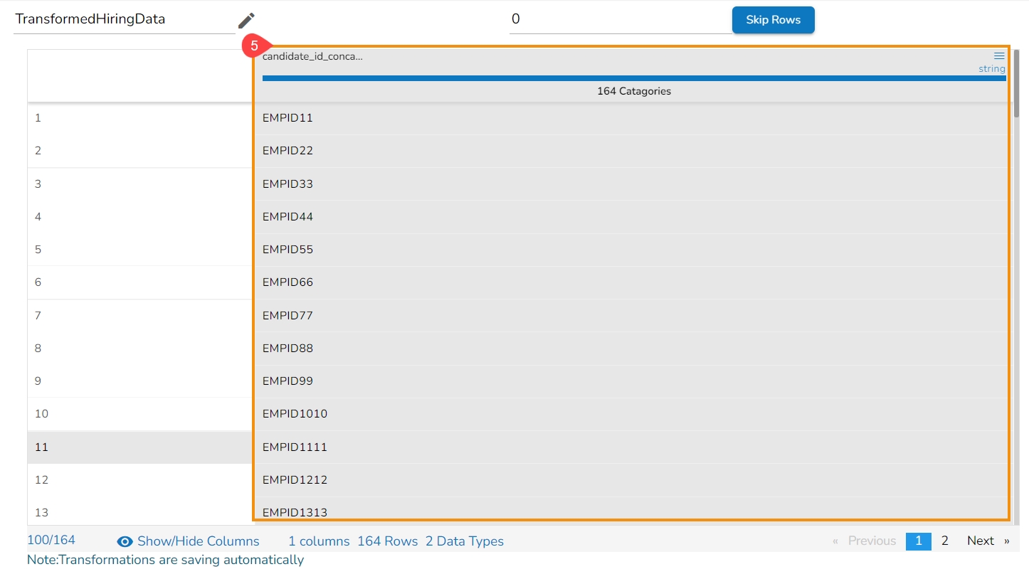
All the other columns except the selected column get deleted.
Please Note: The Delete All Other transform can also be accessed by using the menu icon provided for the each column in the Data Grid display of the dataset.
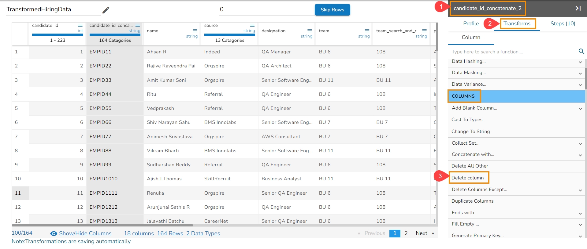
The Delete Column deletes any selected column from the dataset.
Select a column from the dataset within the Data Preparation framework.
Navigate to the Transforms tab.
Select and click on the Delete Column transform from the COLUMNS transform category.
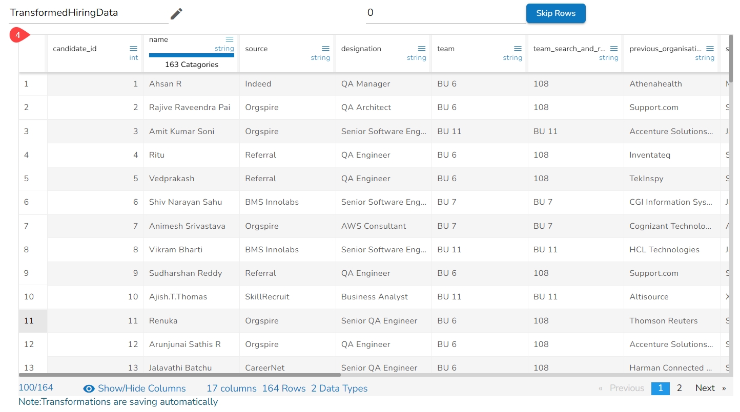
The selected column gets deleted from the dataset.
Please Note: The Delete Column transform can also be accessed by using the menu icon provided for the each column in the Data Grid display of the dataset.
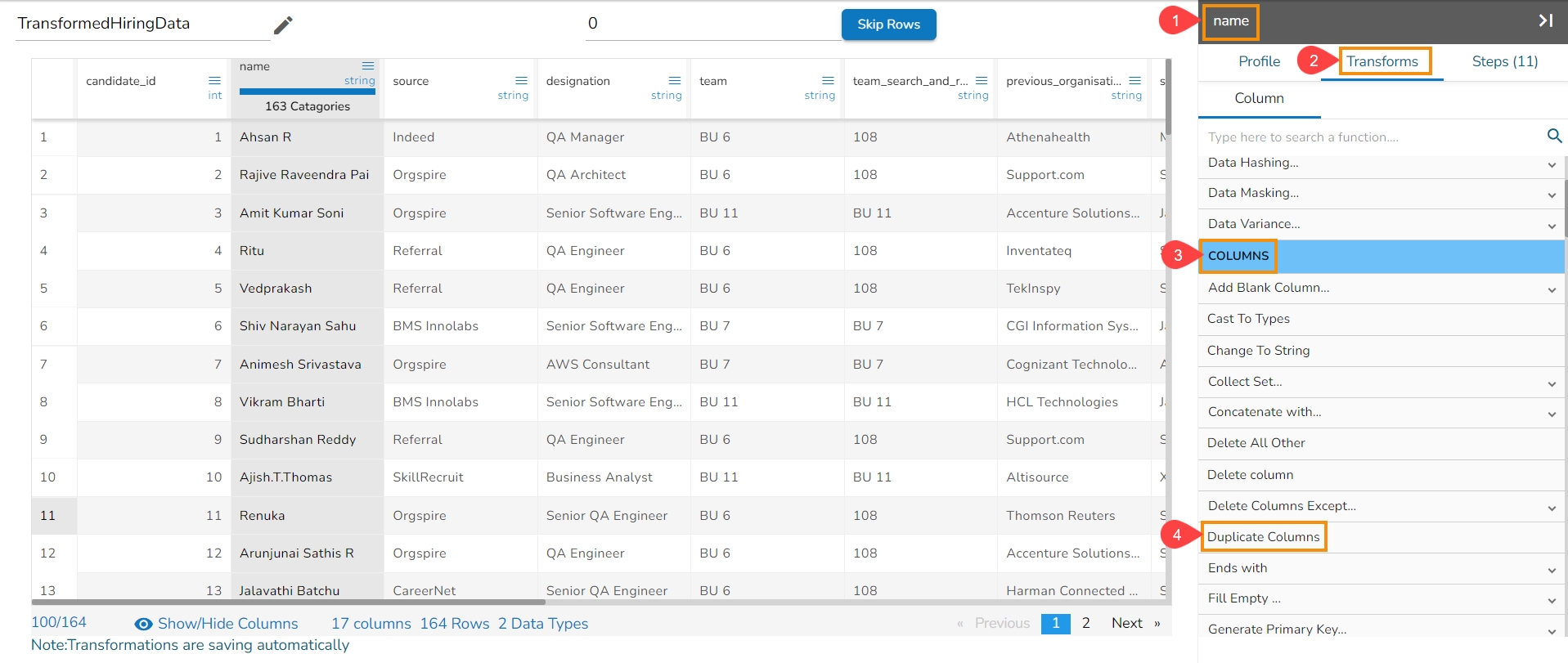
The Duplicate Columns transform creates another column containing the duplicate data of the selected column.
Select a column from the Dataset in the Data Preparation framework.
Open the Transforms tab.
Select and click the Duplicate transform from the COLUMNS category.
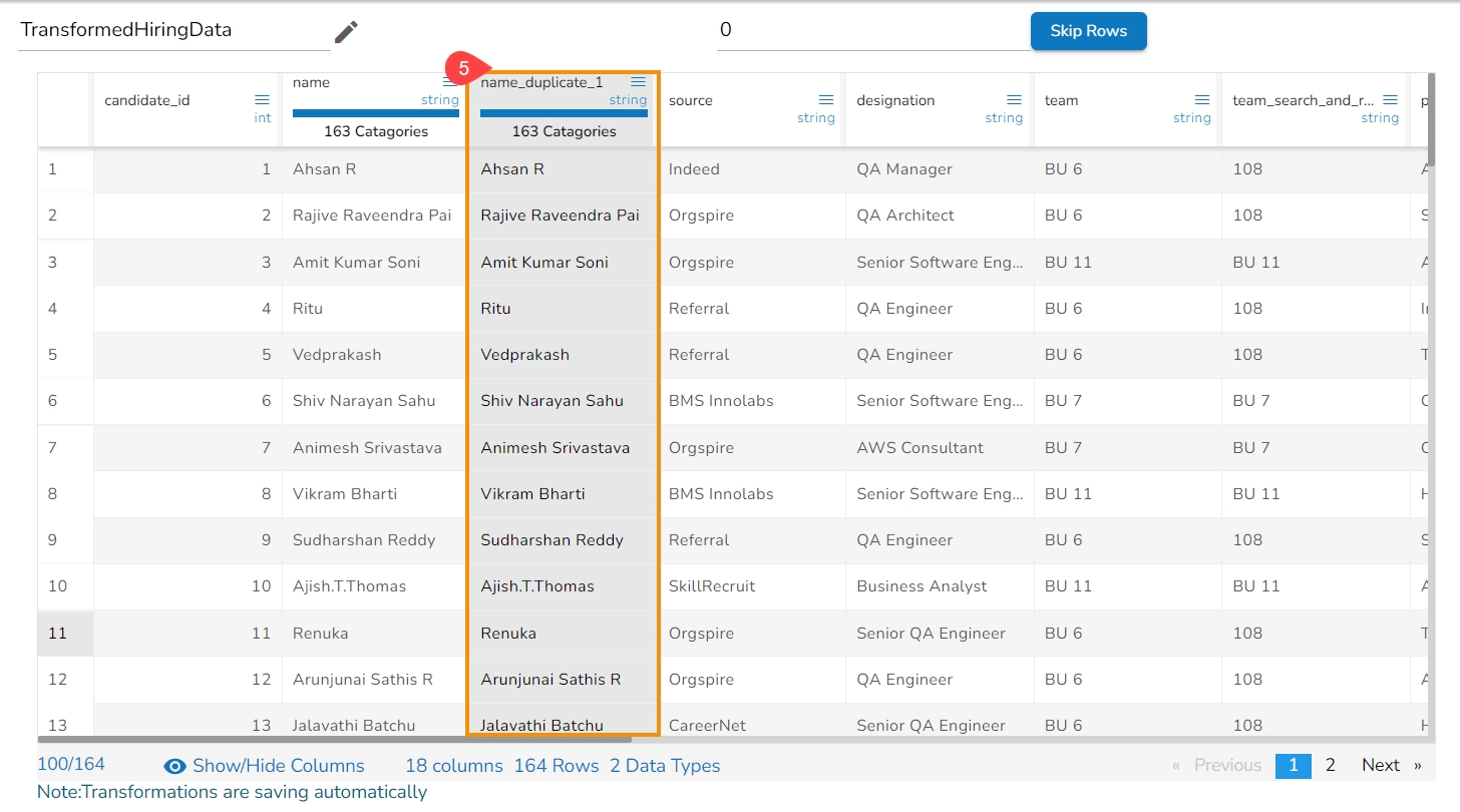
It duplicates the selected column data and inserts it in the dataset.
Please Note: The Duplicate Columns transform can also be accessed by using the menu icon provided for the each column in the Data Grid display of the dataset.
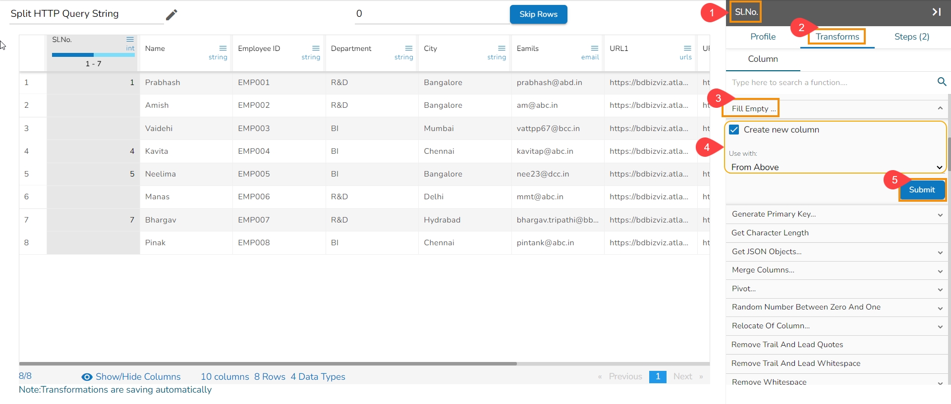
The Fill Empty transform is used to fill the null/empty value of cell using either above or below values available in the column.
Select a column with empty rows from the dataset within the Data Preparation framework.
Open the Transforms tab.
Configure the Fill Empty transform from the COLUMNS category:
Create new column- Click the checkbox to create a new column or else the currently selected column gets updated.
Use with-The user can use either of the options from the provided choices:
From Above: To fill the empty cells and replace them by the value of the cells given above the empty cells.
From Below: To fill the empty cells and replace them by the value of the cells given below the empty cells.
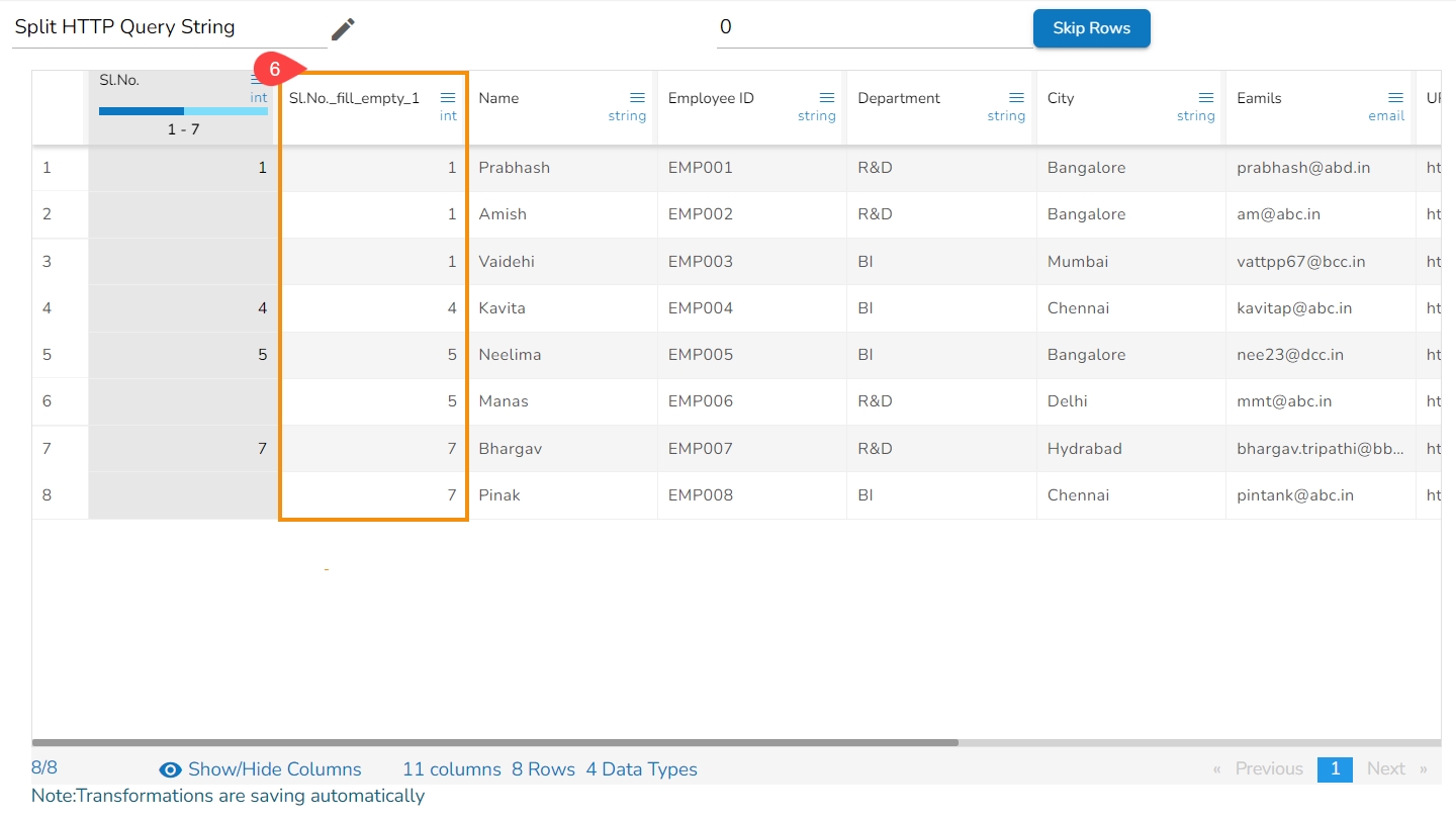
The Fill Empty transform has been applied to the Gender column by filling the empty cells with the values of the immediate below cells.
As a result, a new column gets created with some of the empty cells filled by the values of the immediate below given cells as shown in the below image:
Please Note: The Fill Empty transform fills the immediate empty cell with either above or below cell's values. It does not fill the cells for which both above and below cells are empty.
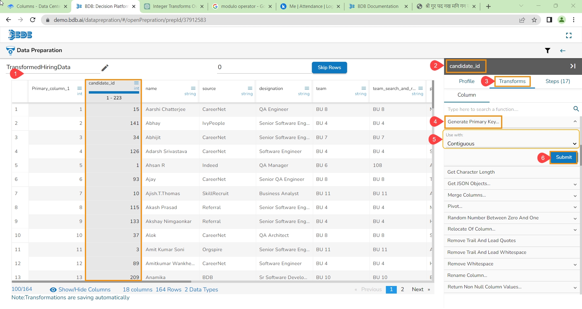
It generates the primary key for the table. The user can see the Primary_column added as the first column in the selected Dataset.
Please Note: Generate Primary Key is a table-based operation.
Navigate to the dataset in the Data Preparation format.
Select the first column from the displayed dataset.
Open the Transforms tab.
Select the Generate Primary Key transform from the COLUMNS category.
Use with: The user gets two options to generate the primary key:
Contiguous- It generates the auto-incremented value starting from 1.
Non_contiguous- It generates a unique and random integer value.
Click the Submit option.
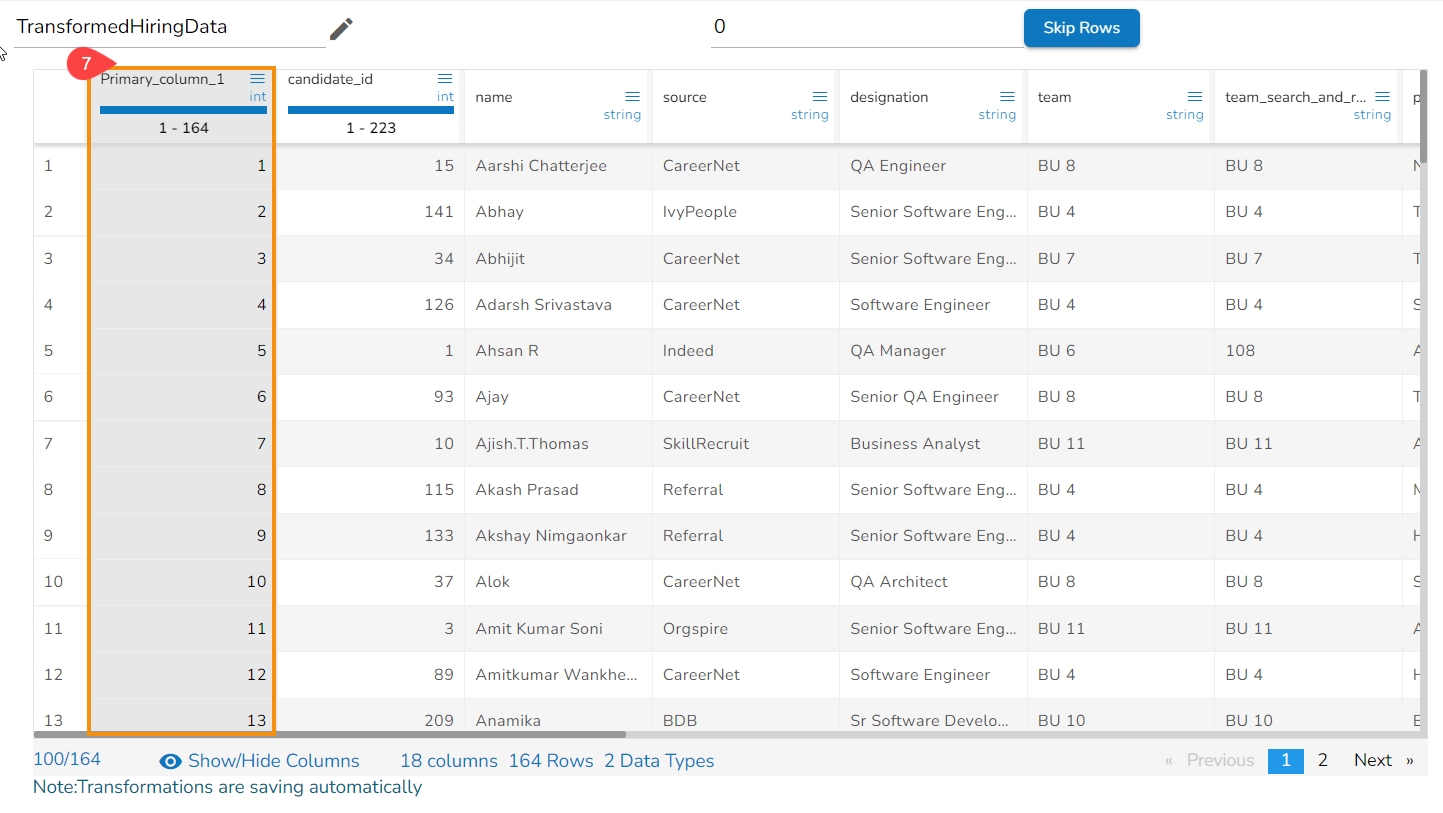
A new column with primary values gets added to the data grid.
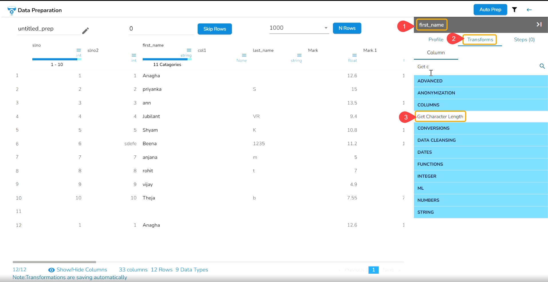
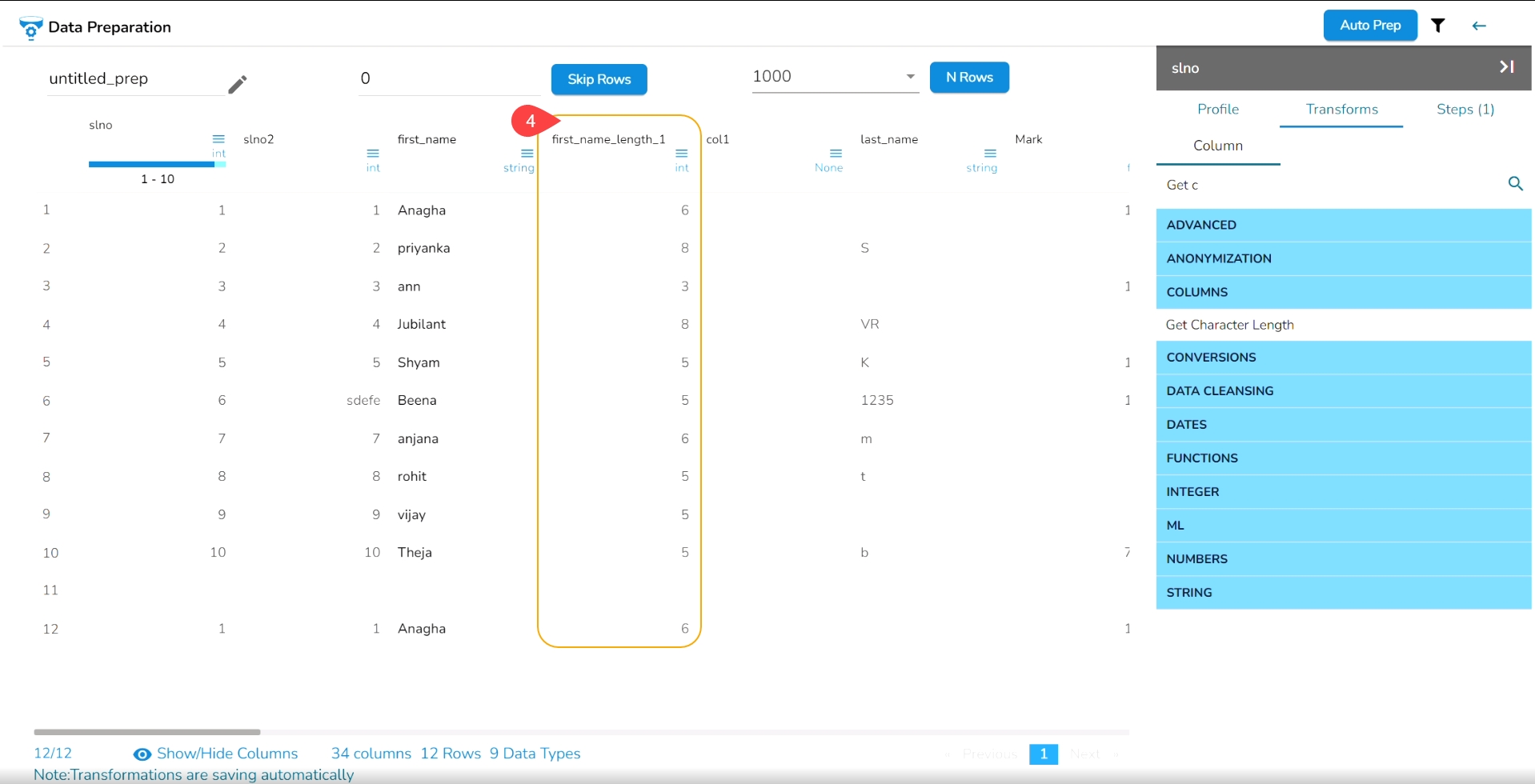
The transform Get Character Length when applied adds a new column with numbers displaying the length of character present in that cell.
Check out the given Walk-through on how to use the Get Character Length Transform.
Select a column from the dataset.
Navigate to the Transforms tab.
Click the Get Character Length transform from the COLUMNS category. E.g., The Get Character Length transform has been applied to the designation column.
As a result, a new column gets added next to the selected column displaying the character length of each cell value as displayed below:
Please Note:
This transform counts the space provided between two words as a character. So, to get the exact count of the character length the cell should not have any space between two words.
The empty cells are kept as it is in the column.
The Get Character Length transform can also be accessed by using the menu icon provided for the each column in the Data Grid display of the dataset.
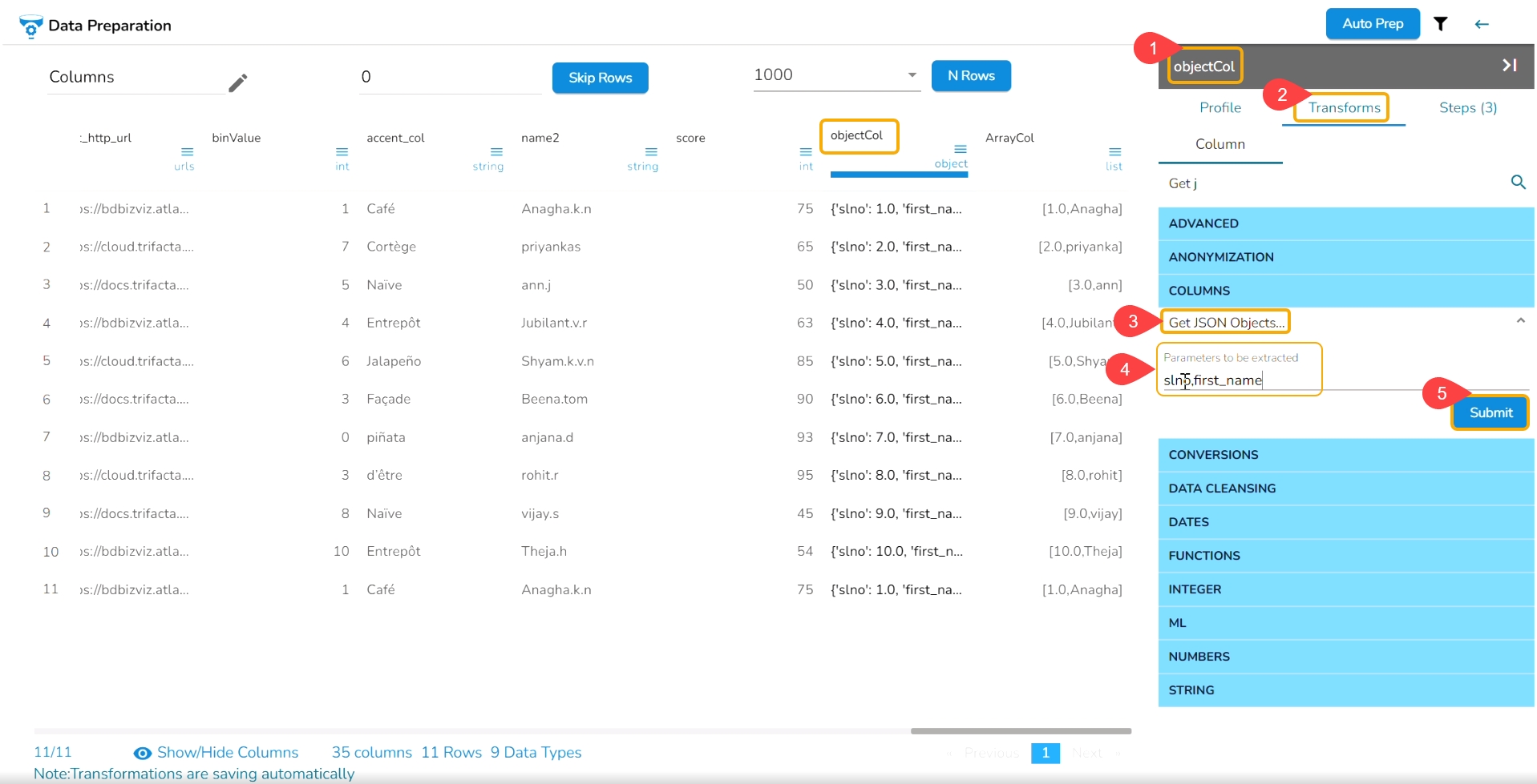
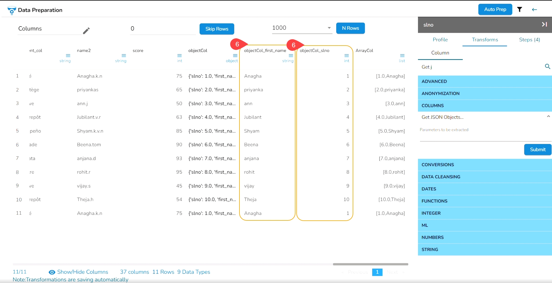
The Get JSON Objects transform extracts any parameter from a given column with JSON data. When the parameter in the JSON is specified, the transform extracts all parameter values as columns into a tabular format.
Check out the given illustration on how to use Get JSON Objects.
Please Note: To extract the nested JSON the ‘,’ mark can be used to specify the multiple values.
Select a column from the dataset within the Data Preparation framework.
Open the Transforms tab.
Select the GET JSON Object transform from the COLUMNS category.
Provide Parameters to be extracted from the selected column.
Click the Submit option.
The given parameters are extracted into tabular structure as displayed-below:
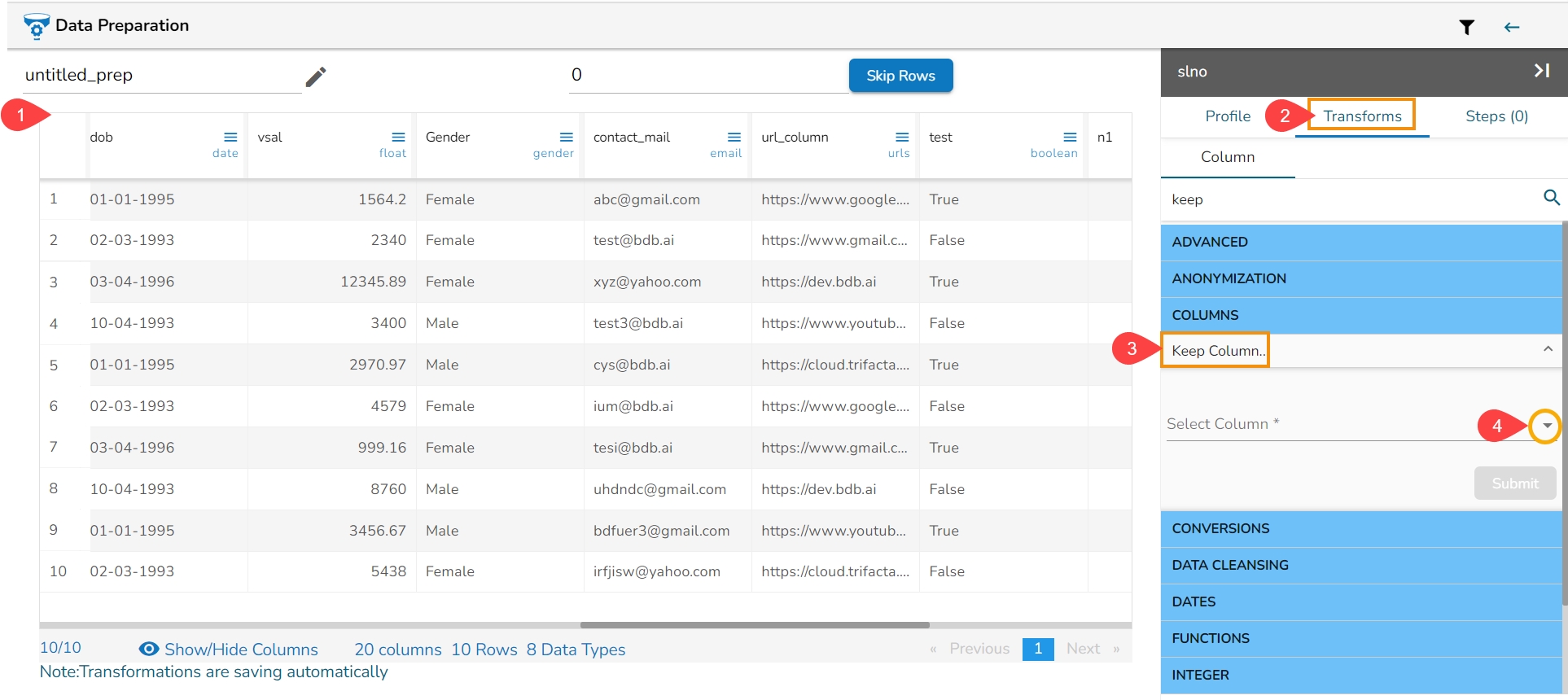
This transform helps the users to keep the selected columns and as a result it deletes all the other columns from the dataset.
Navigate to a dataset in the Grid format within the Data Preparation framework.
Open the Transforms tab.
Select the Keep Column transform from the COLUMNS category.
Click the drop-down icon provided to select columns.
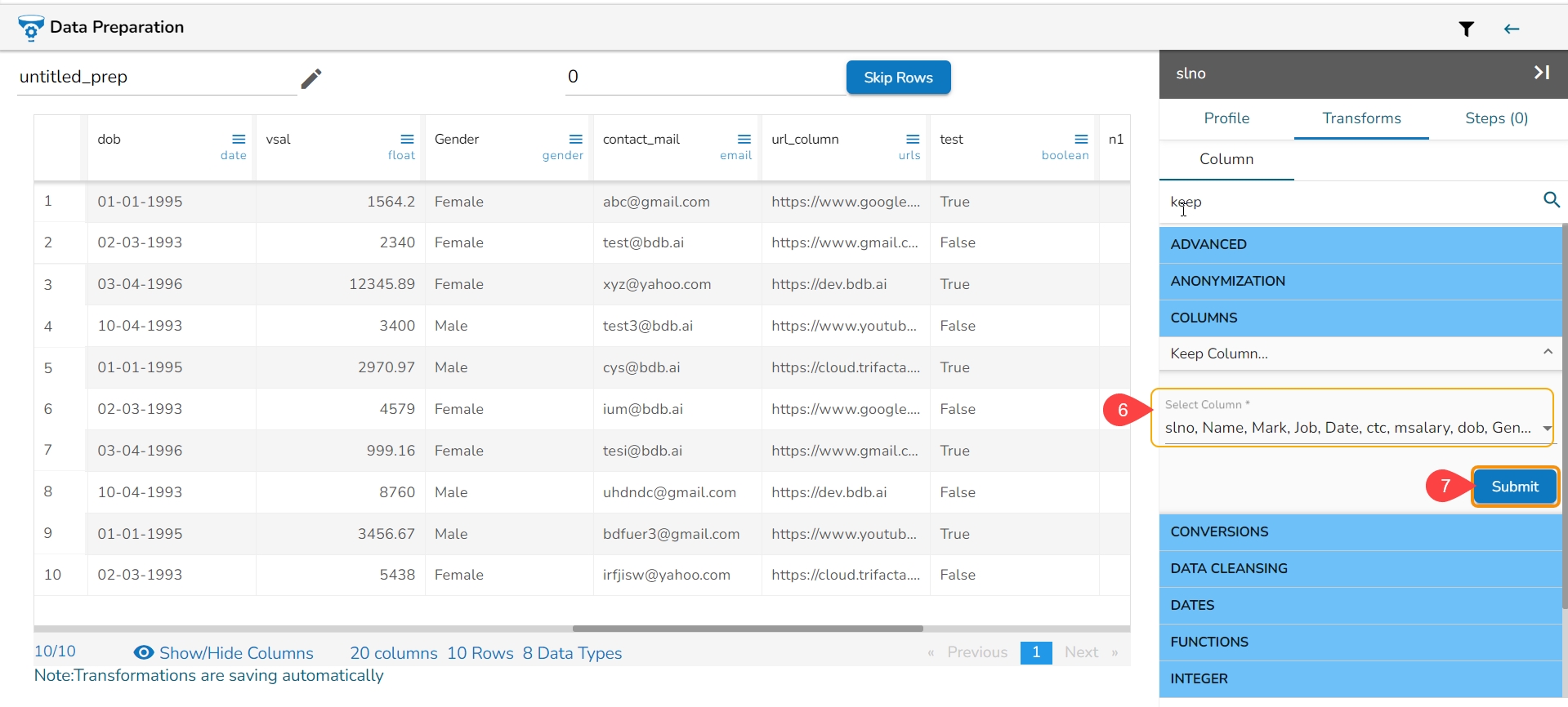
Use check boxes provided next to the column names to select the columns that you want to keep (You can select multiple columns).
The selected columns appear.
Click the Submit option to apply the transform.
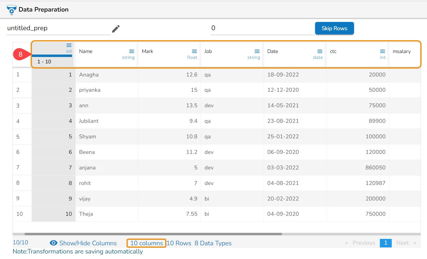
The columns except the selected columns get removed from the Dataset.
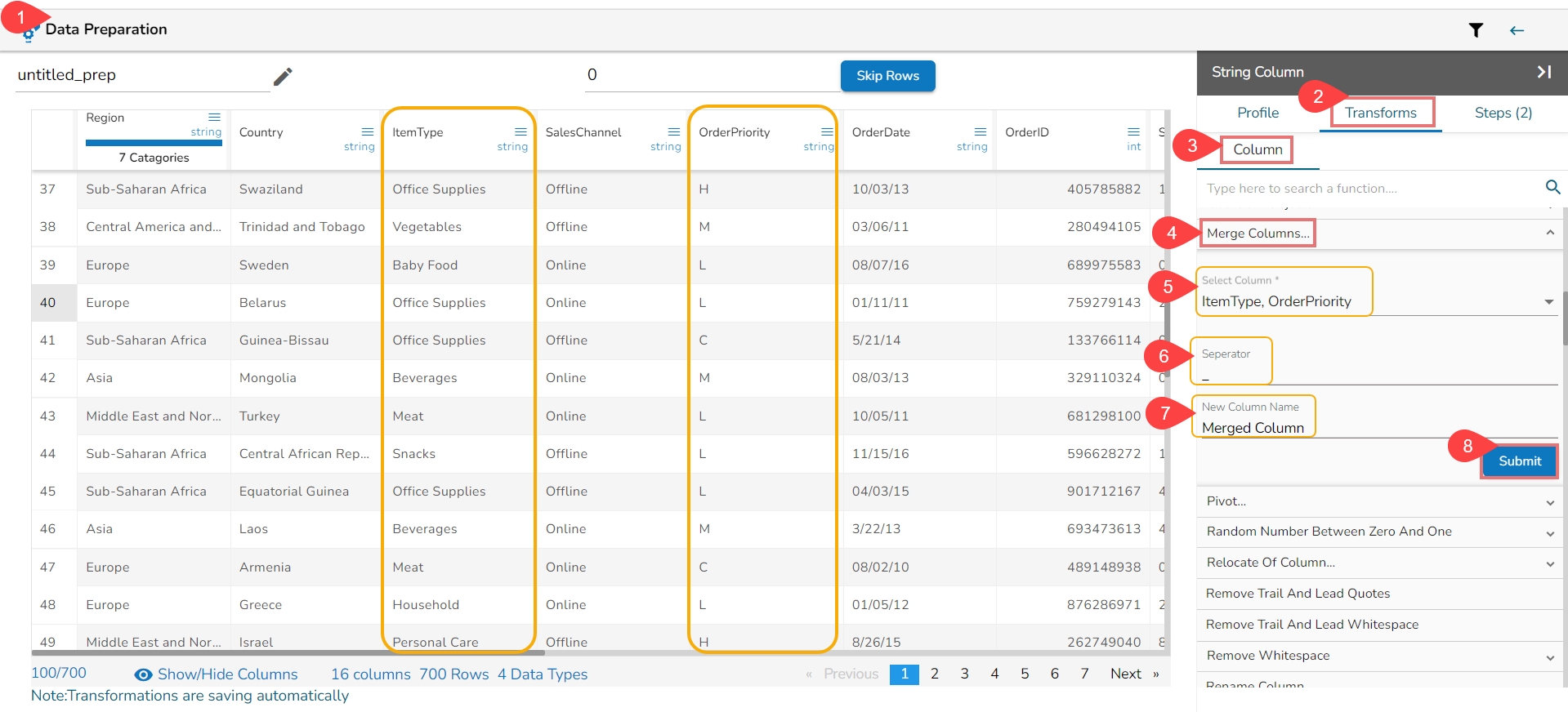
This transformation helps to merge one or more columns and create a new column. By using a separator the values will be separated. E.g., In the following examples the used Separator is '_' (underscore).
Navigate to the Data Preparation grid page.
Navigate to the Transforms tab.
Open the Columns transform type.
Select the Merge Columns transform.
Select the Columns using the Select Columns drop-down menu.
Select a separator.
Provide name for the New Column.
Click the Submit option.
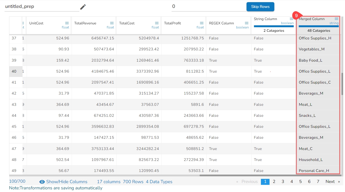
As a result, a new column gets added to the data grid with the merged values of the selected columns.
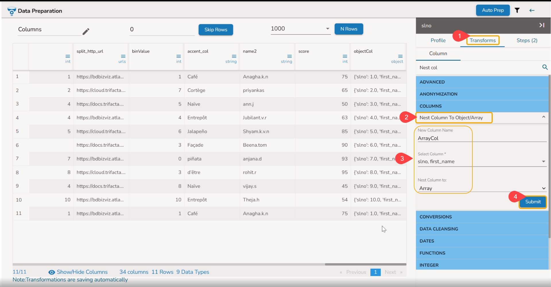
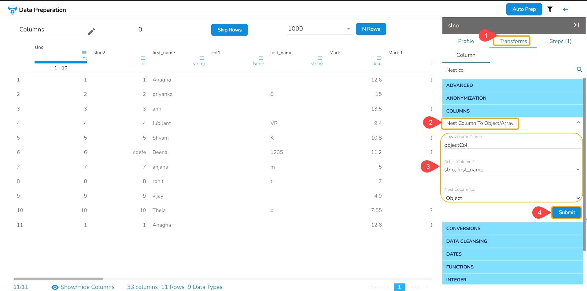
This is nesting one or more columns into an Array or Object column.
Steps to perform the transformation:
Navigate to the Transforms tab.
Select the Nest Column to Object/ Array transform.
Provide the following information:
Provide a name for the new column. It will be the result column.
Select one or multiple columns (The given example displays multiple columns selected).
Select the Nest Column to option as an Object or Array. In the given image, the selected option is Object.
Click the Submit.
Please Note: Based on the selected Nest Column to option, the result will appear:
Array option displays comma separated values in the result column.
Object option displays values within the curly brackets.
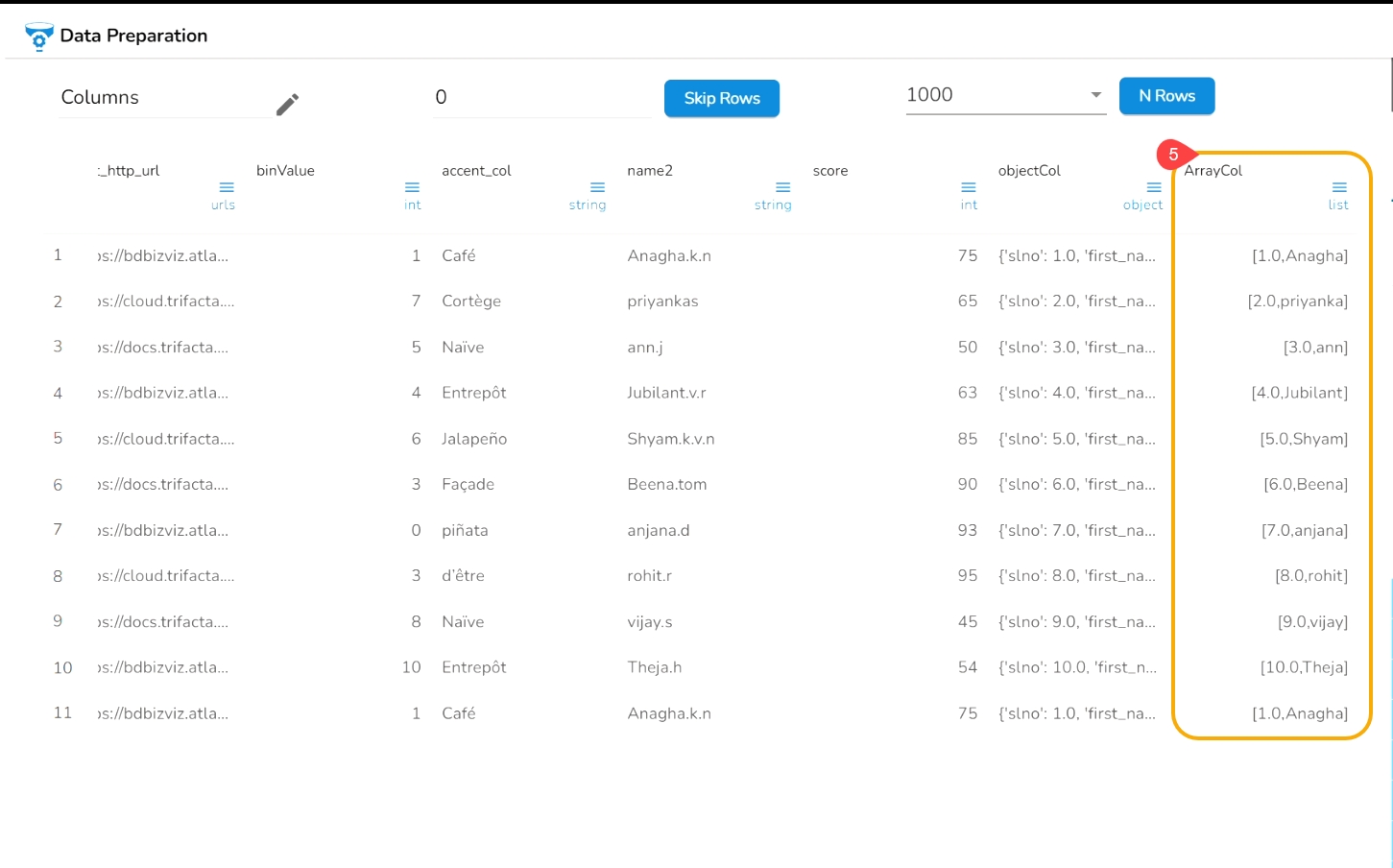
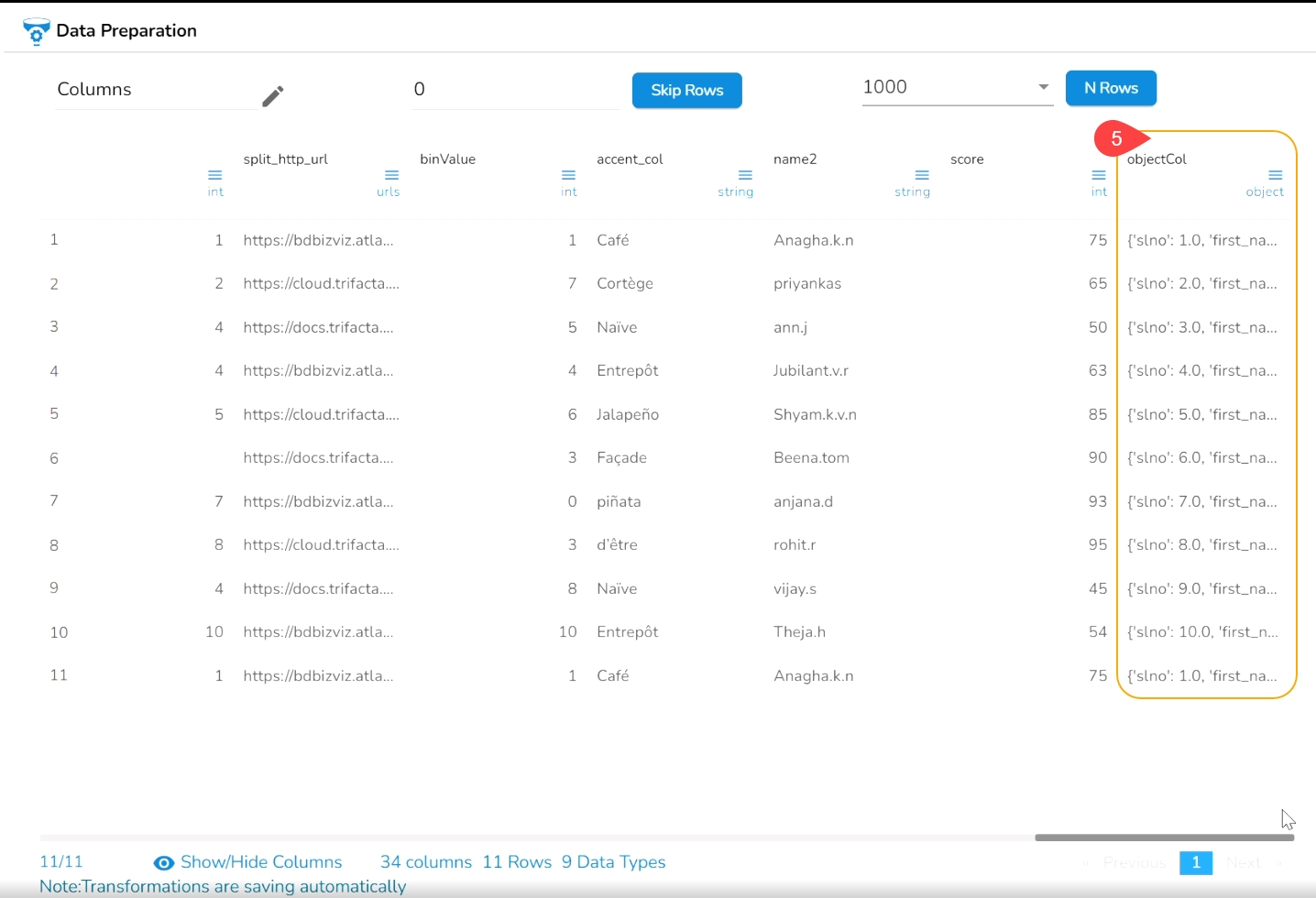
The following images display the result column that appears respectively with the Object and Array as selected option:
Please Note: The result of the Nest column to Array transformation comes as list datatype & this datatype is not supported while loading the data in the datastore.
When applied, the Pivot transform converts the data into a Pivot table based on the selected Pivot Column and Group of the selected columns.
The pivot data transform is a data manipulation operation used to reshape a dataset, primarily in the context of data analysis and data visualization. It involves converting data from a "long" format to a "wide" format, or vice versa, based on the structure of the original dataset.
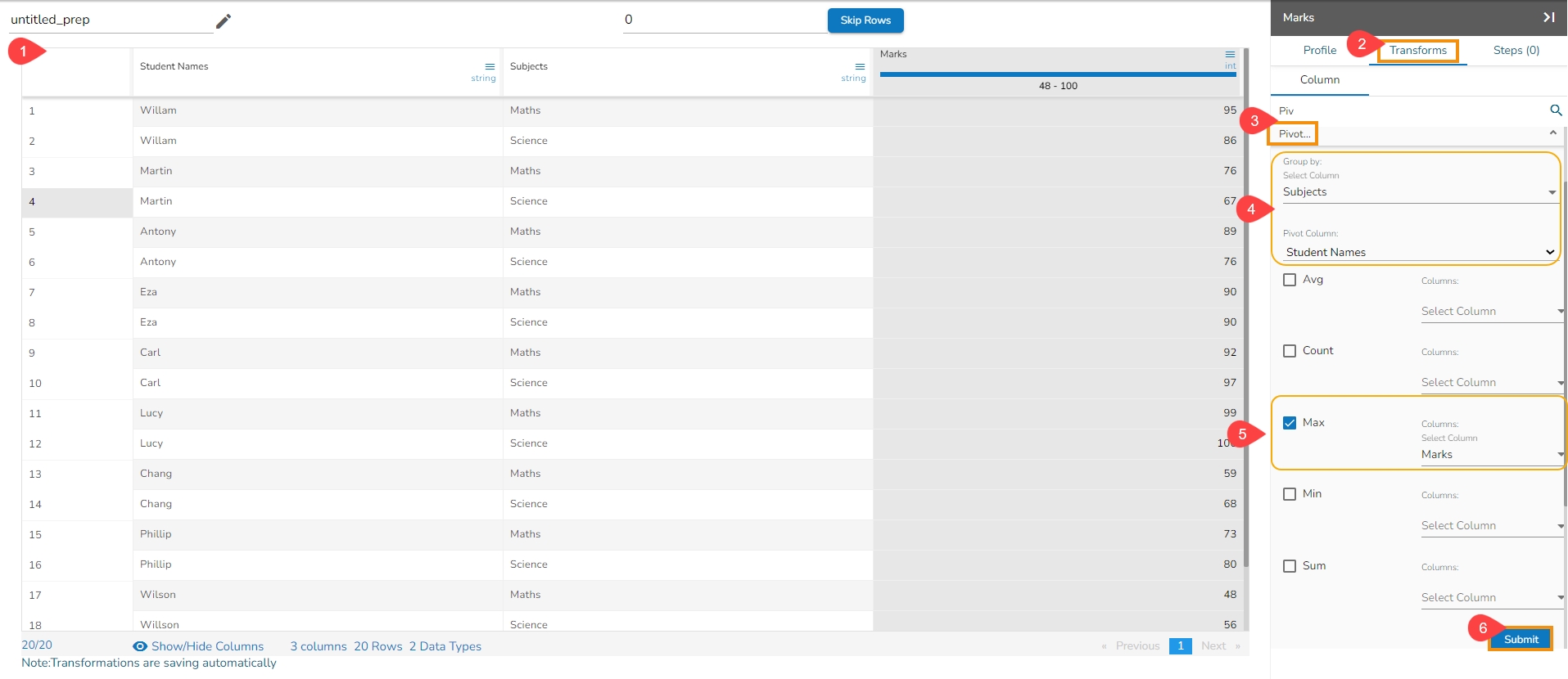
Navigate to the Data Preparation page with a dataset.
Open the Transforms tab.
Select the Pivot transform from the COLUMNS category of transforms.
Select a column to be used for Group By function (It supports String datatype).
Select a Pivot column (It supports String datatype).
Choose an aggregation operation out of Avg, Count, Max, Min, and Sum options with an integer column.
Click the Submit option.
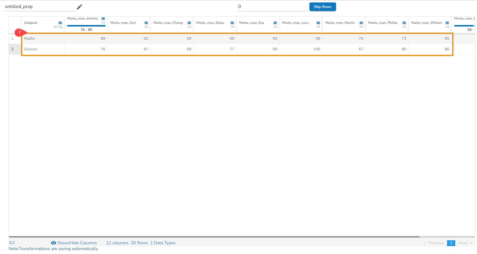
Transform Selection: In the given sample data, the Students Names is selected as the Pivot Column, and Max aggregation is selected for the Marks column. The selected Group by column is Subjects.
As a result, it returns the Max Marks for both the subjects get displayed for each Student in the following manner.
Please Note: The user can change the data display by interchanging the selected columns used for Group by and Pivot.
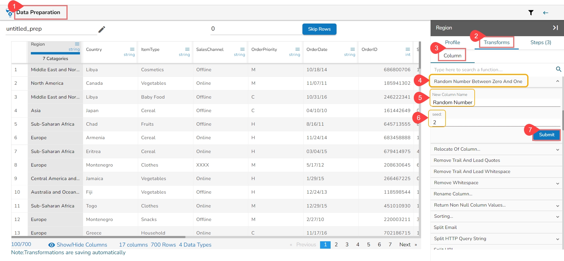
The RAND transform generates a random real number between 0 and 1.
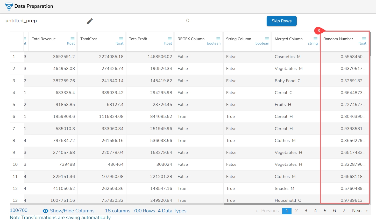
The function accepts an optional integer parameter (seed value), which causes the same set of random numbers to be generated with each execution. When the browser is refreshed, the random numbers remain consistent when the seed value is present.
This function generates values of Decimal type with fifteen digits of precision after the decimal point.
Steps to perform the Random Number between Zero and One transform:
Navigate to the Data Preparation landing page with a dataset.
Open the Transforms tab.
Select the COLUMNS category of transforms.
Select the Random Number between Zero and One transform .
Provide the New Column Name.
Provide seed value (use any integer parameter).
The output will generate random numbers between 0 & 1 in the new column.
Please Note: If none is provided, a seed is generated based on the system timestamp.
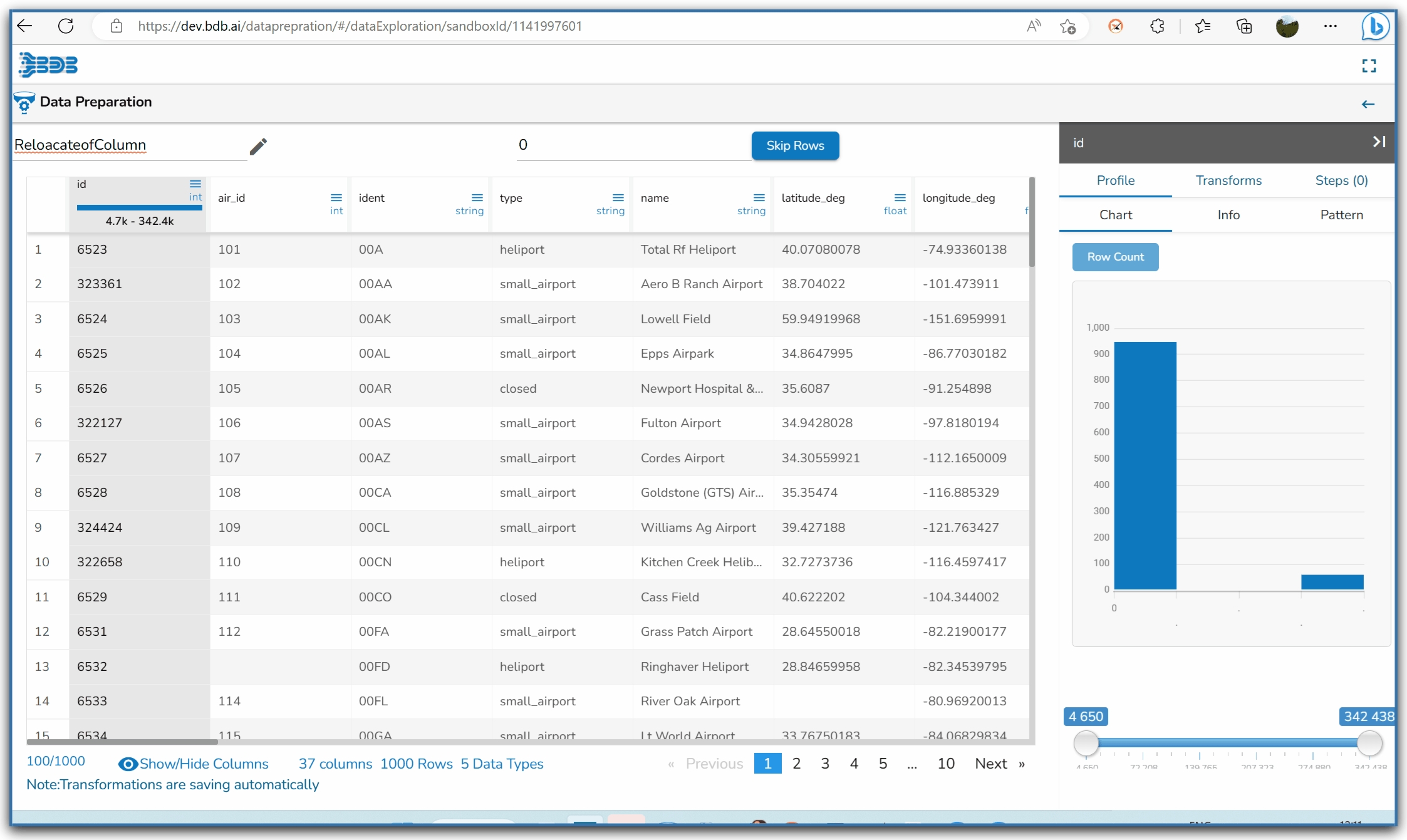
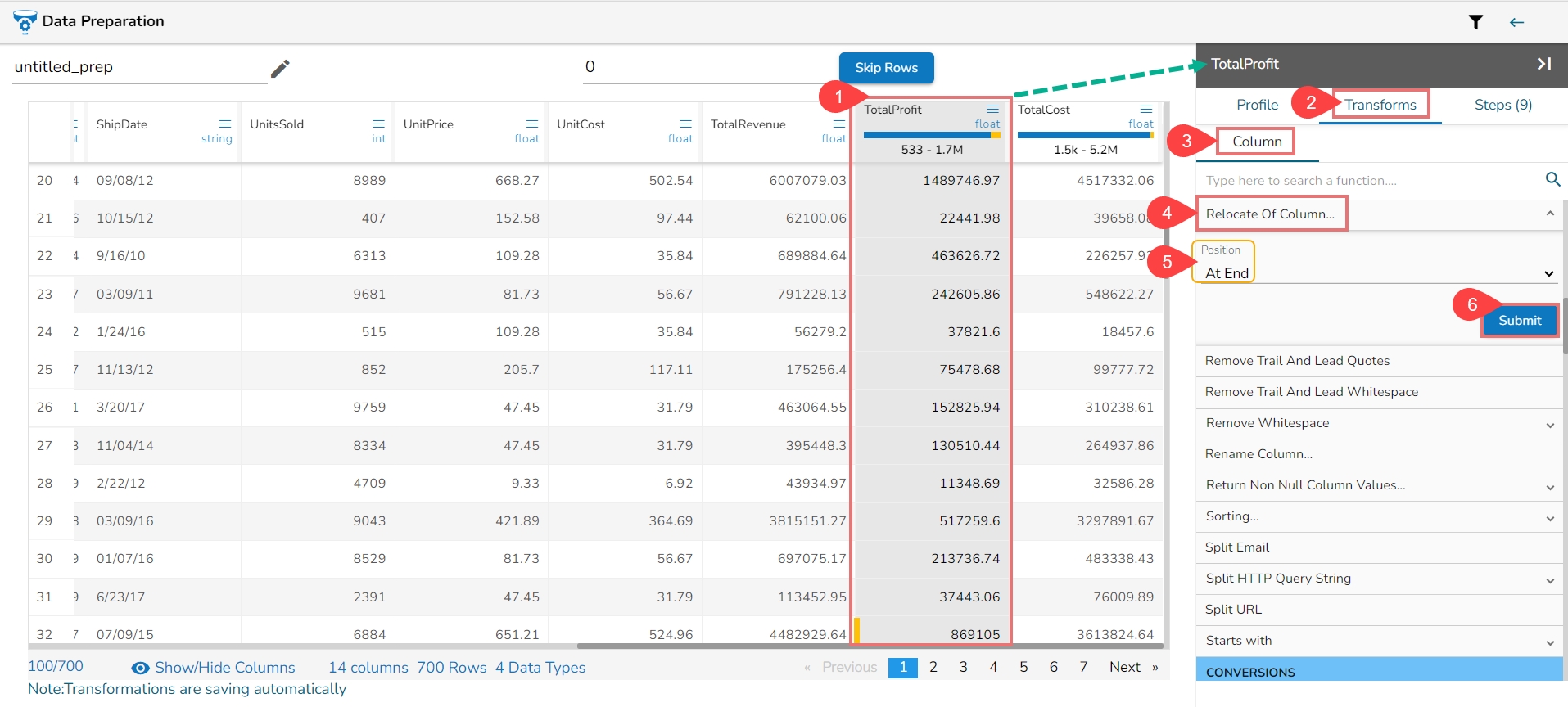
This transform helps to relocate/ change of the position of a column in the data preparation. It will be helpful to the user when there are more columns and the user can change the position as per the given options:
At End
At Start
After Column
Before Column
Steps to perform the Relocate of Column transform:
Navigate to the Data Preparation landing page with a dataset.
Open the Transforms tab.
Select the COLUMNS category of transforms.
Select the Relocate of Column transform .
Select a Position option using the drop-down icon.
The supported positions are: At End, At Start, After Column, Before Column
Click the Submit option.
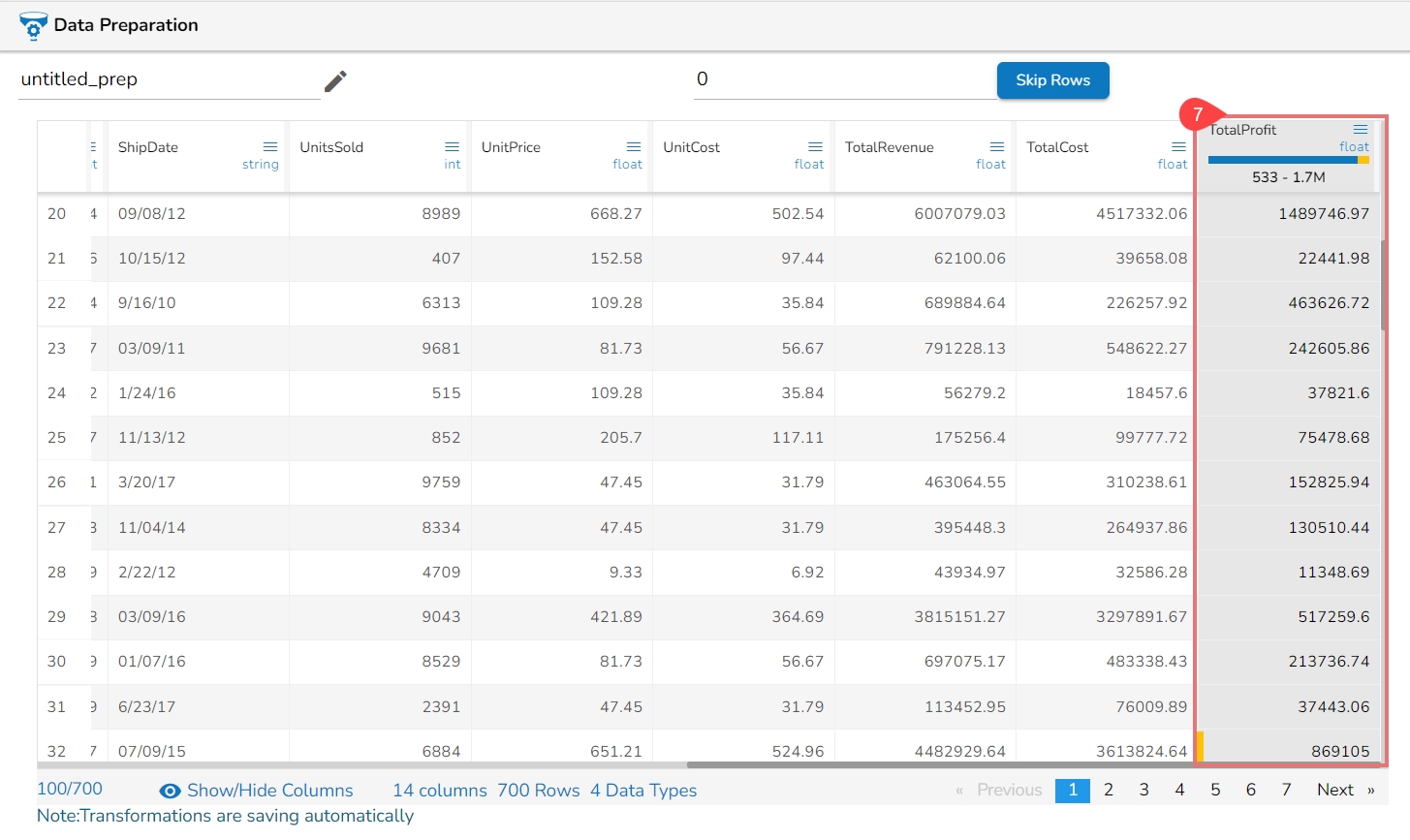
As per the selected position the column gets displayed in the Data Grid.
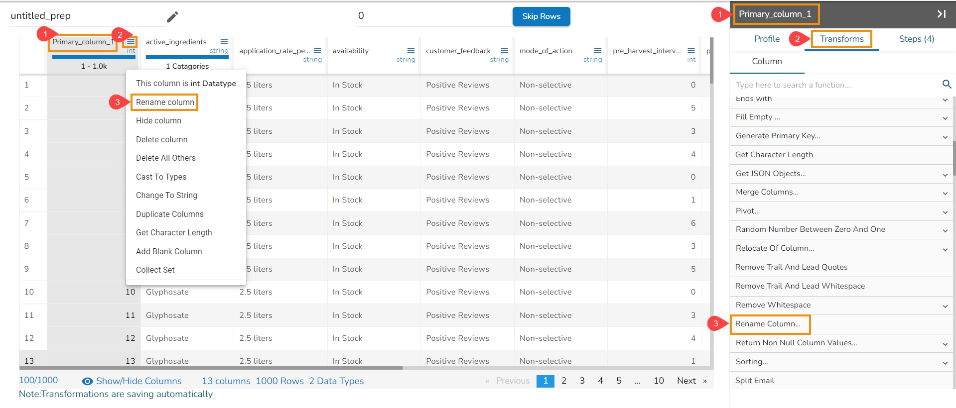
The Rename Column transform allows the user to rename the selected column.
Select a column from the data grid that needs to be renamed.
Open the Transforms tab.
Choose the Rename Column transform.
Or
Select a column from the data grid that needs to be renamed
Click the Menu icon provided next to the Column name.
Select the Rename Column option from the context menu.
The Rename Column dialog box opens (In both the scenarios).
Provide a name that you wish to use as a rename for the selected column.
Click the Submit option.
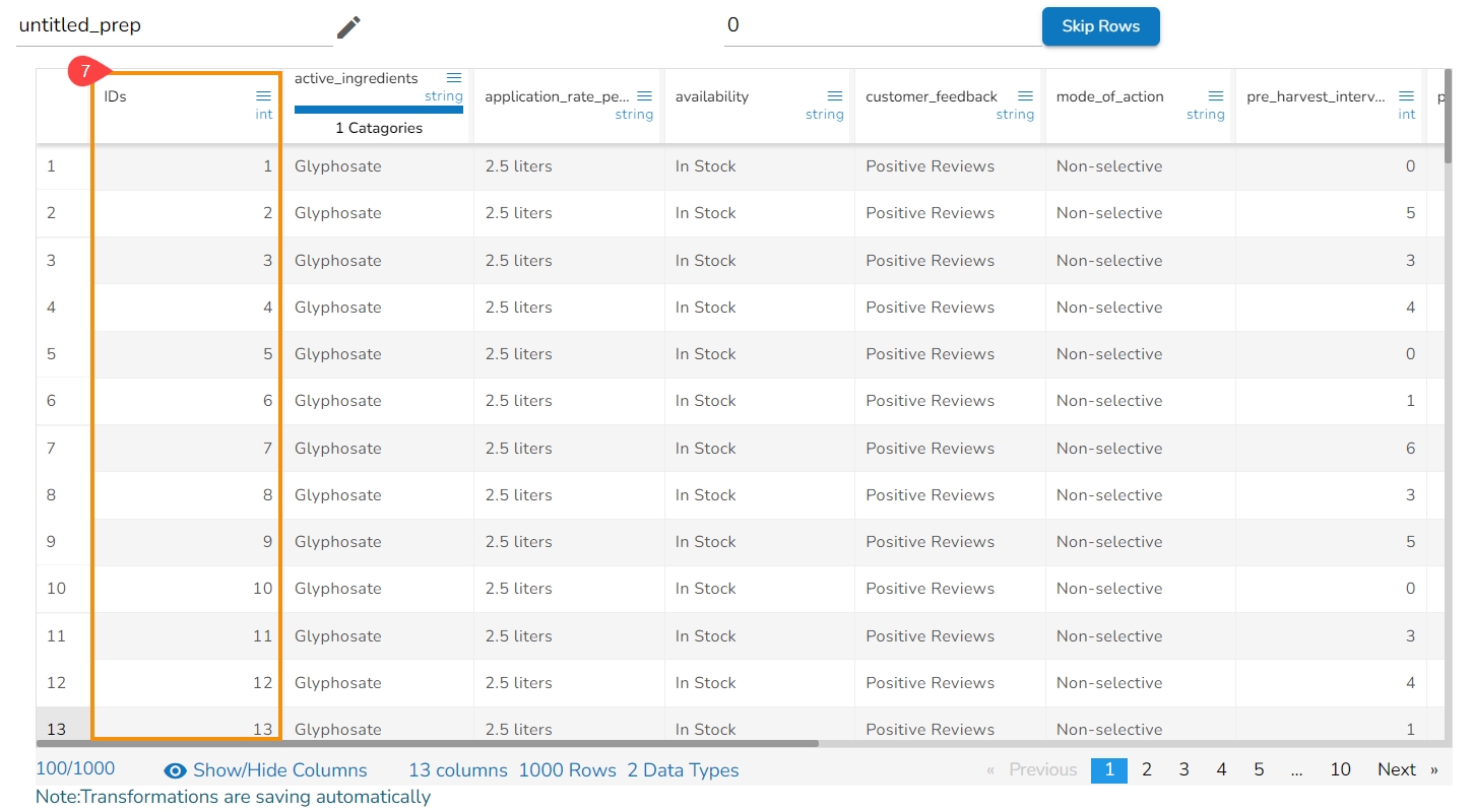
The column gets renamed.
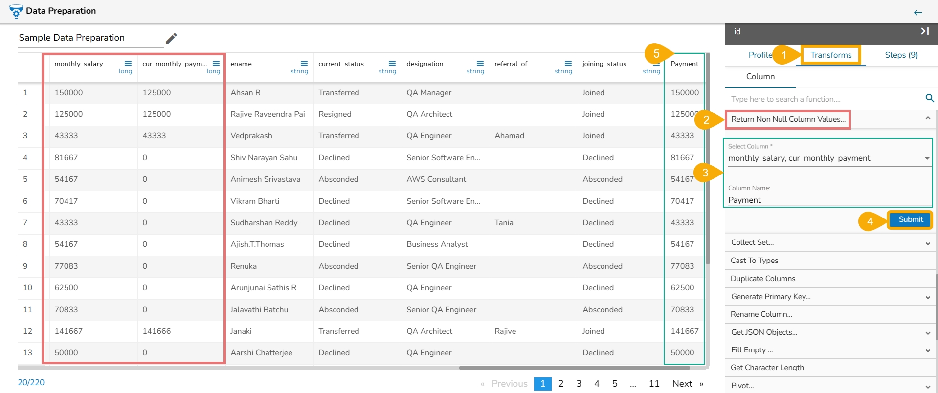
The transform returns the first non-null value from the list of columns specified to a new column. To perform the transform, select the columns which must be checked for null and specify a column name for the result.
Select Column: Select the columns to be checked for null
Column name: The name for the new result column returns
The Return Non Null Column Values transform has been applied to the monthly_salary and cur_monthly_payment columns. As a result, the Payment column gets added to the dataset with the values based on the applied transform.
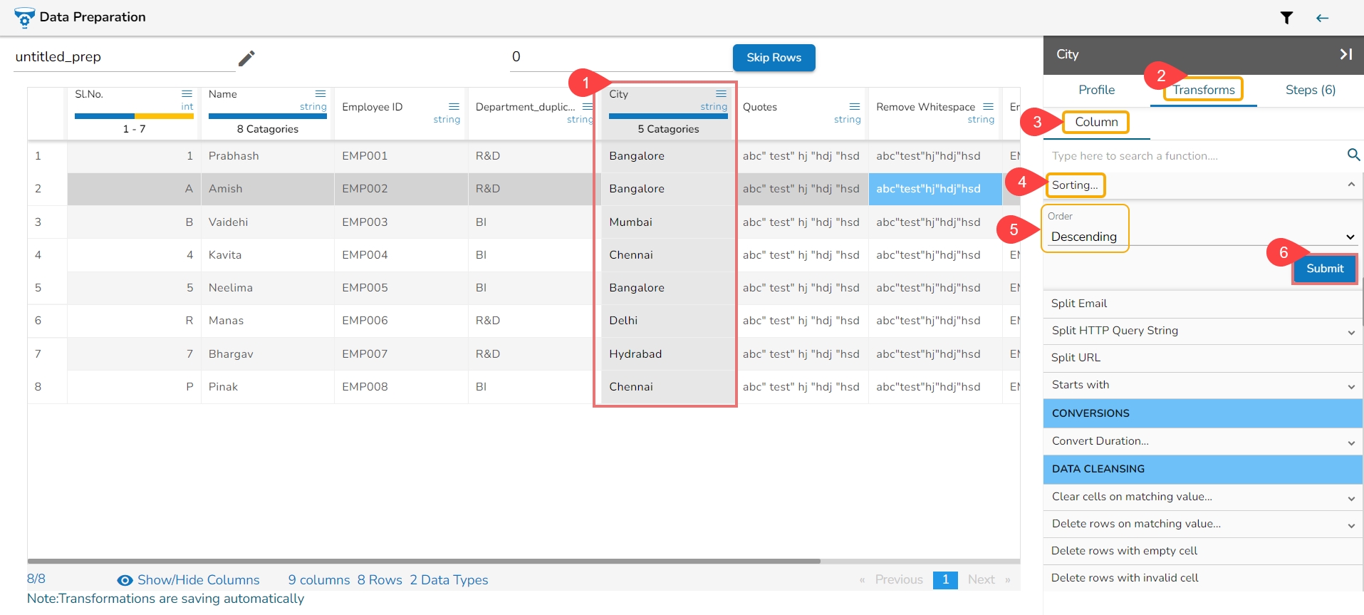
The Sorting transformation helps to sort the column in Ascending/ Descending order for the ease of the user in data preparation. There are two options are given:
Ascending
Descending
Steps to use the Sorting transform.
Navigate to a column using the grid view of the Data Preparation.
Open the Transform tab.
Select the Column transform category.
Click on the Sorting transform.
Select order using the drop-down option.
Click the Submit option.
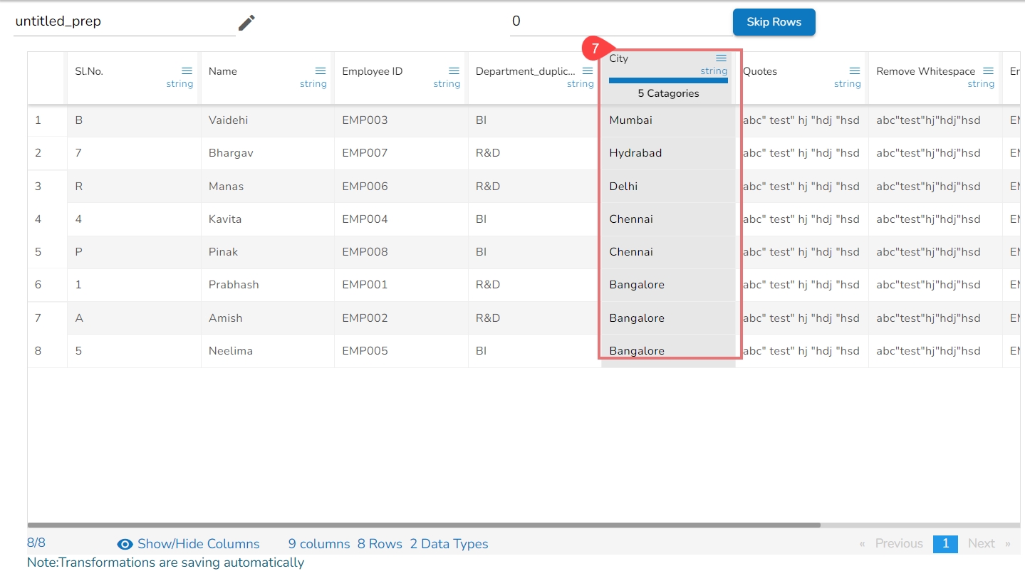
Order of the entire dataset gets changed based on the selected source column.
Please Note: If the Sorting transform is used multiple time, the dataset will be ordered based on the last selected sorting order.
This transform helps to performs arithmetic operation on the selected numerical column.
The Integer data transform performs arithmetic operations on numerical data by applying basic mathematical operations to each data point in a dataset. These operations include addition, subtraction, multiplication, and division. The purpose of these transformations is to modify or manipulate the data in some meaningful way, allowing for easier analysis, visualization, or computation.
Addition (+): This operation involves adding a constant value to each data point in the dataset. It can be useful for tasks such as shifting the data along the axis or adjusting the data to a new reference point.
Subtraction (-): Subtraction subtracts a constant value from each data point. Like addition, it can be used to shift the data, but in the opposite direction.
Multiplication (): Multiplication scales each data point by a constant factor. It can stretch or compress the data along the axis, altering its magnitude.
Division (/): Division divides each data point by a constant value. It can be useful for normalizing the data or expressing it in relative terms.
Modulus(%): Modulus divides the given numerator by the denominator to find a result. In simpler words, it produces a remainder for the integer division.
These arithmetic operations can be performed on individual data points or entire datasets. The operations are straightforward and commonly used in data processing and analysis.
For example,
When dealing with sensor readings, you might add a constant offset to calibrate the measurements.
In financial analysis, you might multiply data by a scaling factor to adjust for inflation or currency conversions.
Check out the given walk-through on how to use the Addition, Subtraction, and Multiplication options under the Integer transform.
Steps to use the Integer Transform:
Select a numerical/ Integer column from the dataset.
Open the Transforms tab.
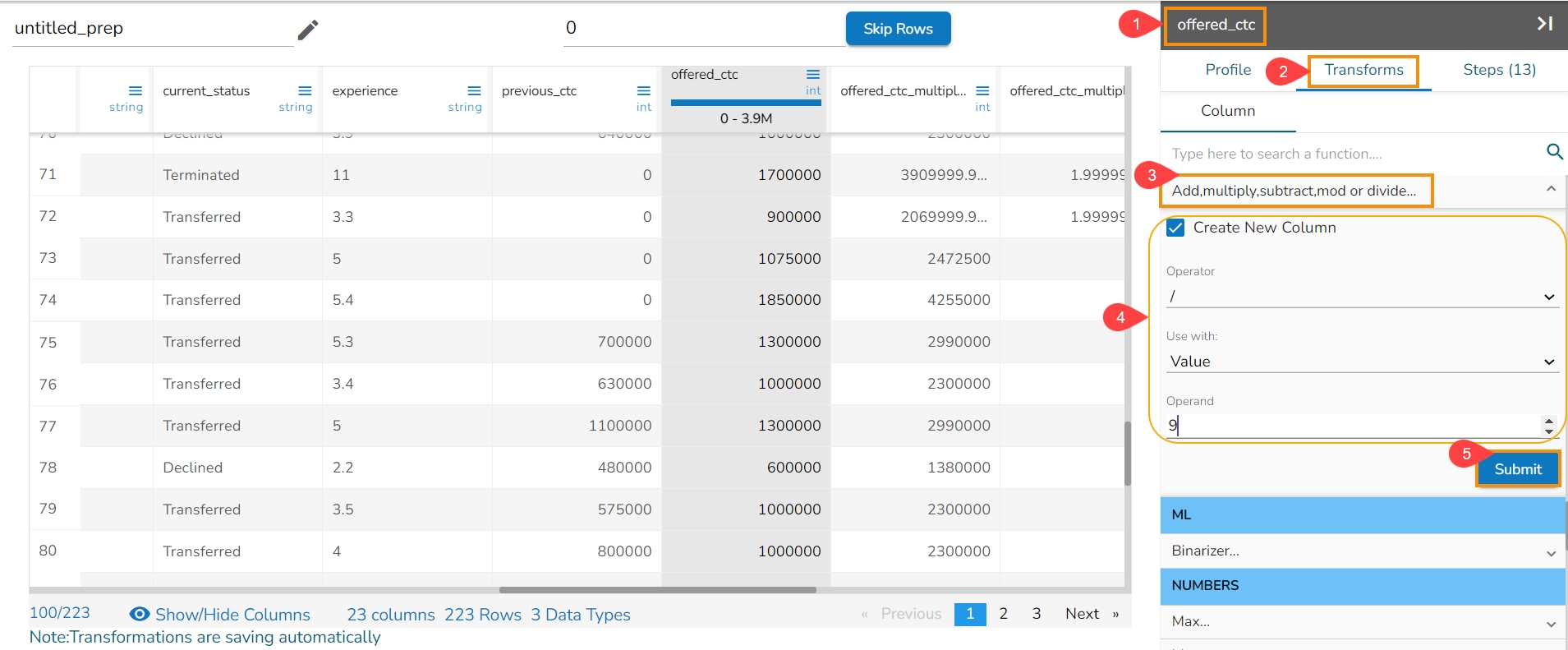
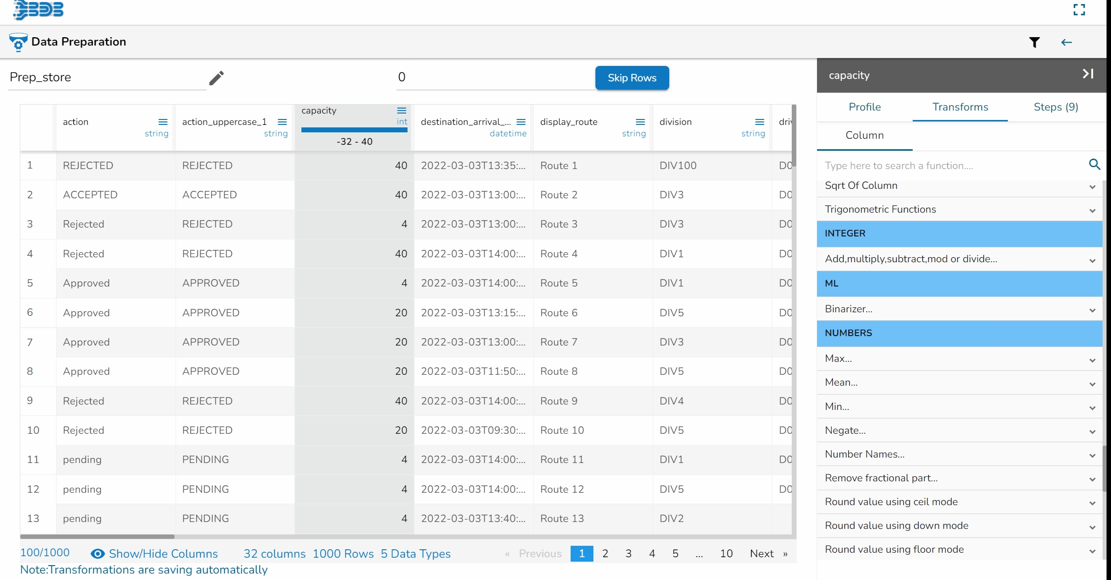
Select the Add, multiply, subtract, mod, or divide transform provided under the Integer category.
Operator: There are five arithmetic operations to choose ( +, -, / , *, %). Select any one operator.
Use with: The operation can be performed between two columns and to a column based on a value.
Operand/Column: The arithmetic operation needs an operand if it is to be used with a value.
The arithmetic operation needs another column if the selected Use With option is Column.
The first operand is one on which the operation is being performed. The second operand can either be a value or other numerical column based on the choice of use with an option.
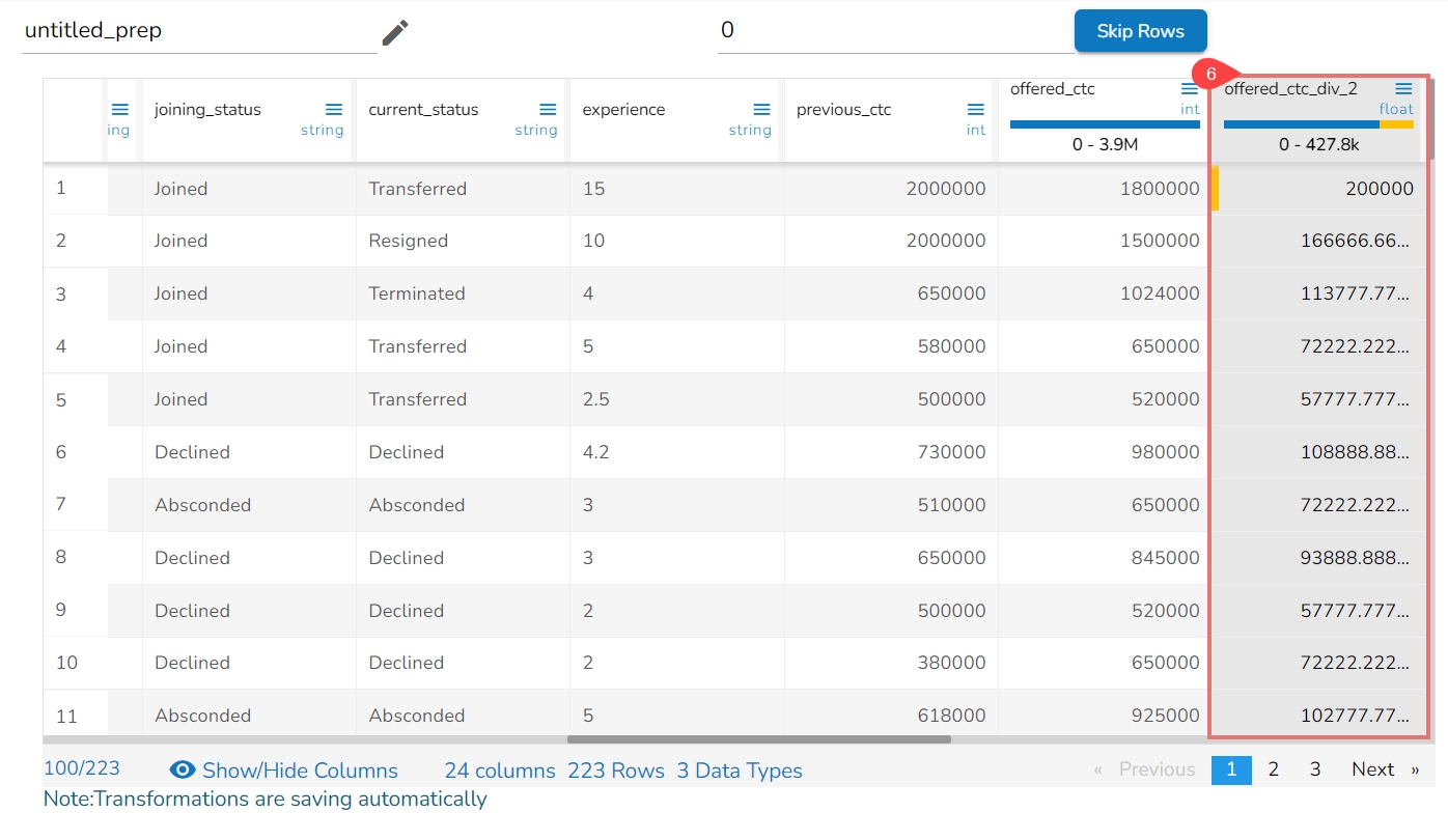
The Integer transform has been applied on the Sales column by choosing division with value where operand is 9.
As a result, a new column gets added with the divided values of the sales.
This transformation also returns the modulo value, which is the remainder of dividing the first argument by the second argument. Equivalent to the Modulus (%) operator.
Steps to perform the transformation with the Modulus (%) operator.
Select the required column in which MOD should calculate.
Select Create New column (optional).
Set the Operator as MOD (%).
Use with Value or Other Column.
Pass the value or select the other column.
Result will come in a new column in which MOD returns the remainder of the value.
The Add Prefix transform allows for the effortless incorporation of custom text at the outset of each value. The seamless integration of personalized text at the beginning of each value empowers you to enhance and customize your data in a user-friendly manner.
Check out the given illustration on how to use the Add Prefix transform.
Steps to perform the Add Prefix transformation:
Navigate to the Data Preparation workspace.
Select the Transforms tab.
Open the Add Prefix transform from the String column category.
The Add Prefix dialog box opens.
Provide the following information:
Enable the Output Column Prefix option to add a new column with the transformed values.
Pass the Prefix Value that is needed.
Select one or multiple columns where the prefix needs to be added.
Click the Submit option.
The result will come as a nw column or on the same column by adding the prefix value on the selected columns.
Implementing the Add Suffix transform enables the effortless inclusion of custom text at the end of every value. This transformative technique offers a user-friendly approach to enrich and modify the original data, allowing for the seamless integration of personalized text at the end of each value. By leveraging the flexibility of the Add Suffix transform, you can tailor and enhance your data with ease, ensuring it aligns perfectly with your specific requirements and desired outcomes.
Steps to perform the Add Suffix transformation:
Navigate to the Data Preparation workspace.
Open the Transforms tab.
Select the Add Suffix transform from the String transform category.
Provide the following information:
Enable the Create new Column (Optional) to add a new column with the result data. The Suffix will be added to the same column if this option is not enabled.
Pass the suffix value that is needed.
Select one or multiple columns where the suffix needs to be added.
Click the Submit option.
The result will come as a new column (as in the current scenario) or on the same column by adding the suffix value on the selected columns.
The Change to Lowercase transform converts the values from the selected column into lowercase. This transform can replace the existing column value or add a new column alongside the original data. This flexibility allows for seamless integration and customization of the transformed values within your dataset, giving you the option to either update the existing column or introduce a new column with the lowercase representation of the data.
Check out the given walk-through on how to use the Change to Lowercase transform.
Navigate to the Data Preparation workspace.
Select a column from the displayed dataset.
Select the Transforms tab.
Click the Change to Lower Case transform from the String category.
The Change to Lower Case dialog box opens.
Enable the Create new column option using the checkbox. If this option is not enabled, the data will be changed in the same column.
Click the Submit option.
The result column in the dataset:
The Change to Title Case transform converts the selected column value into title case, resulting in a transformed value where the first letter of each word is capitalized. This transformed value can either replace the existing column value or be added as a new column within the dataset. This flexibility empowers you to smoothly incorporate the title case representation of the data, allowing for enhanced readability and consistency.
Check out the given illustration on how to use the Change to Title Case transform.
Steps to use the Change to Title Case transform:
Navigate to the Data Preparation framework.
Select a column from the displayed dataset.
Open the Transforms tab.
Select the Change to Title Case from the String category.
The Change to Title Case dialog box opens.
Enable the Create a New Column option.
Click the Submit option.
The selected column values get changed into the title case. The Title Case column has been added to the displayed dataset.
Enable the Create a New Column option using the checkbox. Provide a name for the result name. If this option is not enabled, the data of the original column will be modified into the title case.
The Change to Upper Case transform is a data manipulation operation that converts the selected column value to capital letters. This transformation can be applied in two ways: by replacing the existing column value or by adding the transformed value as a new column.
Check out the given illustration on how to use the Change Upper Case column.
Steps on how to use the Change to Upper Case transform:
Navigate to the Data Preparation workspace.
Select a string column from the Dataset.
Open the Transforms tab.
Select the Change to Upper Case transform from the String category.
The Change to Upper Case dialog box appears.
Configure the following details.
Enable the Create a New Column to display the result.
Provide a name to the newly created column with the Upper case data.
Click the Submit option.
Please Note: The data of the selected column will be modified in the same column, if the Create a New Column option is not enabled.
The result column gets added displaying the data in the upper case.
The Ends with transform is ideal for matching values based on patterns for the String data type.
It returns true if the rightmost set of characters of a column of values matches a pattern.
The source value can be a String data type, and the pattern can be a Pattern, regular expression, or a string.
Check out the illustrations on how to use the Ends with transform.
Steps to perform the Ends with transform:
Navigate to the Data Preparation workspace.
Select a String column using the Data Grid.
Navigate to the Transforms tab.
Select the Ends with the transform from the String category.
The Ends With dialog box appears.
Use the drop-down icon to select a mode. The given choices for mode are REGEX and String.
Provide the following information based on the selection:
Provide a name for a new column if the Create New Column option is enabled.
Pass a specific value from the selected column for the 'REGEX' or 'String' mode.
In the REGEX mode, the ends with values can be put. For example, to search through data with the value 'Orgspire', just the letters '.* pire' will be enough.
The String mode requires the entire value from the selected column to be searched through the data.
The Ignore Case option can be used to make string comparison case-insensitive.
Click the Submit option.
The result column will display the values 'True' or 'False' by checking the words in the selected column that end with the given pattern.
All the values that end with the 'pire' pattern will display True in the newly added column with the REGEX mode.
It will also display True for the rows with the "Indeed" value with the String mode).
The Extract Substring at Position transform allows you to extract a portion of a selected column based on the starting position and the length of the substring to be extracted. The transformed value can replace the existing column value or be added as a new column.
Here's how the transform works based on the provided parameters:
Position: This option helps to set the position from where the string is to be extracted.
For example, if the position is 2, the extraction will begin from the third character.
Length: The number of characters to extract from the string is set using the Length field.
Let's see an example:
Suppose there is a column named "Text" with the value "Hello, World!".
When the substring extraction transform is applied by replacing the existing column value and setting the position to 2, the transformed value will be "llo, World!" because it starts from the third character onward.
Please Note
Check out the illustration on how to use the Extract Substring at Position.
Steps to apply the Extract Substring at Position transform:
Navigate to the Data Preparation workspace.
Select a String column with longer values using the Data Grid.
Navigate to the Transforms tab.
Select the Extract Substring at Position transform from the String category.
The Extract Substring at Position dialog box appears.
Provide the following information:
Enable the Create a New Column option.
Provide a name for the newly added column.
Set a number referring to the position from where the value is to be subtracted.
Set a number defining the length of the extracted substring.
Click the Submit option.
A new column will be added to the data grid based on the extracted substring values as per the provided information.
Please Note:
The string column index is set from 0 onwards for the positive numbers, so the first letter will be position 0.
The selected column will be modified to display the substring values as per the set configuration, if the Create a New Column option is not enabled.
The Extract Substring before the Delimiter transform allows you to extract a substring from a selected column based on the count of occurrences of a delimiter. It creates a new column that contains the extracted substring.
Check out the illustration on how to use the Extract Substring before the Delimiter transform for a string column.
Delimiter: Provide the delimiter that separates the substring in the selected column.
Count: It defines the count before the delimiter from where the extraction should happen.
The count of occurrences of the delimiter before which the extraction should happen. This value is mandatory.
Steps on how the transform works based on the provided parameters:
Navigate to the Data Preparation workspace.
Select a string column with at least a delimiter from the Dataset.
Navigate to the Transforms tab.
Select the Extract Substring before Delimiter transform from the String category.
The Extract Substring before Delimiter dialog box opens.
Provide the following information:
Enable the Create a New Column option.
Provide a name for the newly created column (Only if the Create a New Column option is enabled).
Specify the Delimiter.
Provide a digit to specify the Count.
Click the Submit option.
The result column will be added to the Dataset with the extracted substring value as per the set count before delimiter.
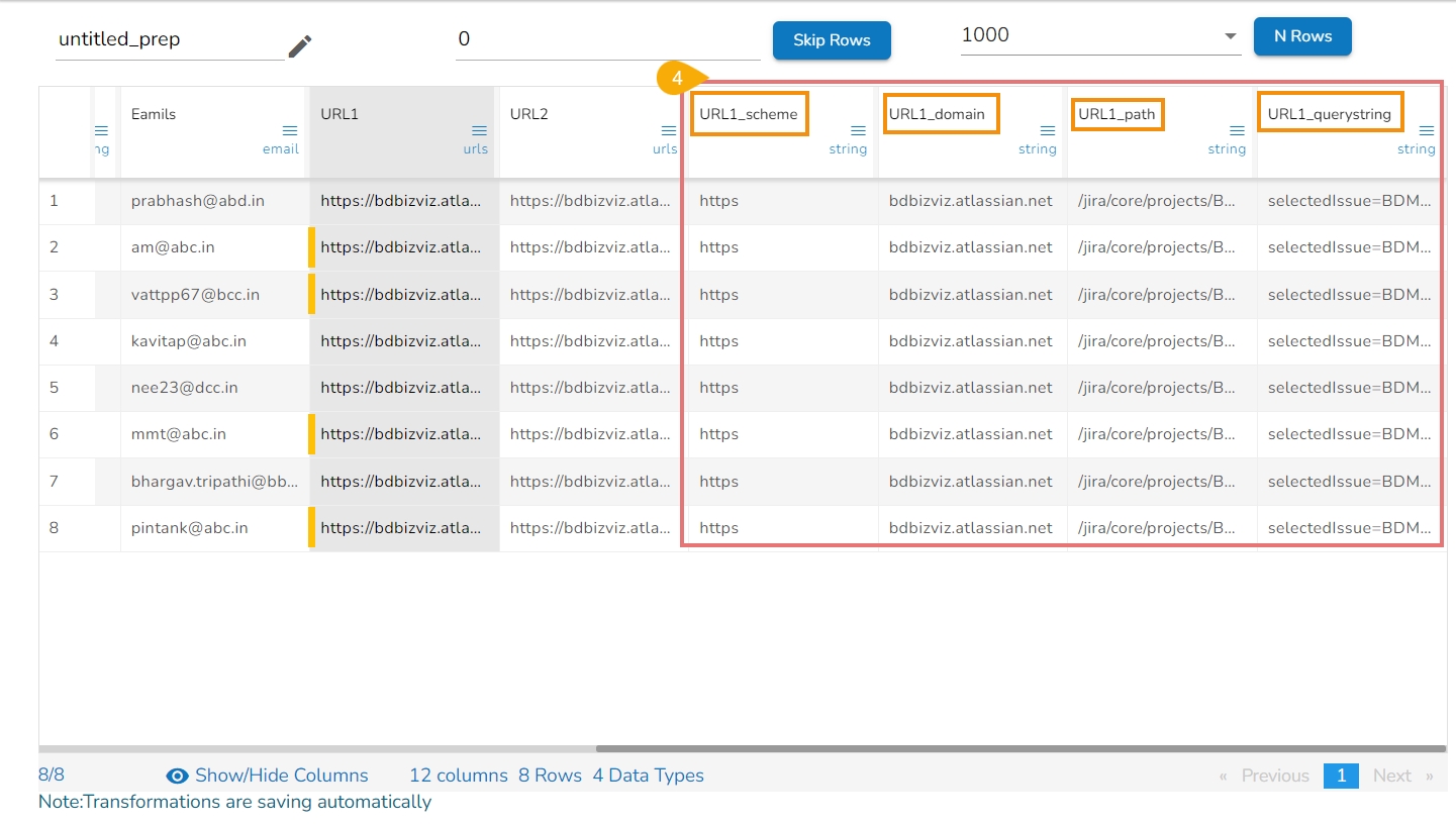
Get Domain Transform extracts the domain from a valid URL. This transform allows you to retrieve the domain portion of a URL, which can be used to replace the existing column value or add the extracted domain as a new column.
Check out the illustration on how to use the Get Domain transform.
Here's how the Get Domain transform works:
Input: The selected column containing the URLs from which you want to extract the domain.
Output: The transformed value will be the extracted domain, which can replace the existing column value or be added as a new column.
Let's see an example of how this transformation works:
Steps to use the Get Domain transform:
Navigate to the Data Preparation workspace.
Select a column containing URL addresses.
Open the Transforms tab.
Search and click the Get Domain transform.
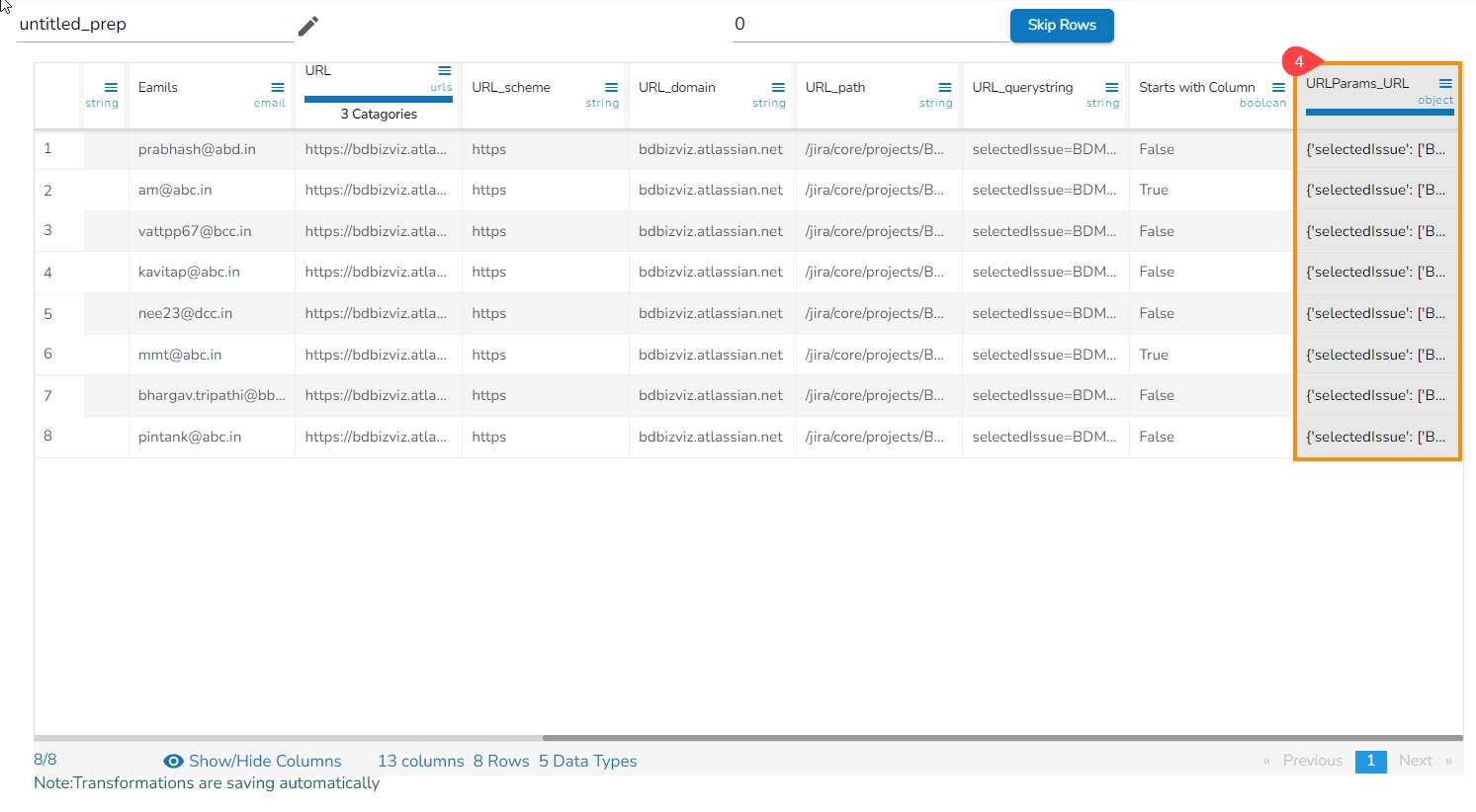
A new column gets added with the extracted Domain from the concerned URLs.
The Get Host transform is designed to extract the hostname from a URL, including the subdomains but excluding the path and query parameters. It helps to isolate the host from the complete URL.
Here's an example to demonstrate how the Get Host transform works:
Check out the walk-through on how to use the Get Host transform.
Steps to use the Get Host transform:
Navigate to the Data Preparation workspace.
Select a column containing URL addresses.
Open the Transforms tab.
Search and click the Get Host transform.
A new column gets added with the extracted Host IDs from the concerned URLs.
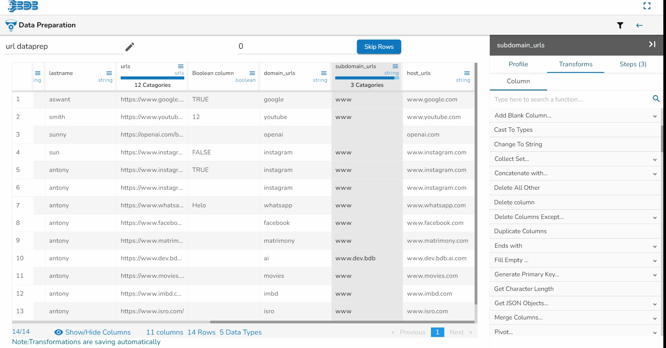
Use the Get Subdomain Name transform to extract the subdomain name from a valid URL.
Here's an example to demonstrate how the Get Subdomain Name transform works:
Check out the illustration on how to use the Get Subdomain Name Transform.
Steps to use the Get Subdomain Name transform:
Navigate to the Data Preparation workspace.
Select a column containing URL addresses.
Open the Transforms tab.
Search and click the Get Subdomain Name transform from the String category.
A new column with the subdomain names gets added to the Data Grid view of the dataset.
The Insert Character transform allows you to insert a character after a specified position in a cell value. This transformation can either replace the existing column value or add the modified value as a new column.
Check out the illustration on how to apply the Insert Character transform.
Here's how the Insert Character transform works based on the provided parameters:
Navigate to the Data Preparation workspace.
Select a column from the dataset.
Open the Transforms tab.
Select the Insert Character from the String category.
The Insert Character dialog box appears.
Provide the following details to apply the Insert Character transform.
Enable the Create a New Column option using the checkbox.
Provide a name for the newly added column (applicable only if the Create a New Column option is enabled).
Position: The position(s) in the cell value after which the character should be inserted. You can specify a single position or multiple positions as comma-separated values.
Character: The character that should be inserted after the specified positions.
Click the Submit option.
The Insert Character transform has been applied in the below-given column to the esalary column. The selected position is 0, and the character to be added is $:
The result column displays the data with the inserted character. Data of the selected source column can be modified, or a new column will be entered with the inserted character.
The Negate Boolean Value transform is a data manipulation operation that returns the opposite value of a given Boolean value. It negates or flips the Boolean value from True to False or False to True.
Please Note: It supports the Boolean column where True/ False values are mentioned.
Check out the illustration on how to apply the Negate Boolean Value transform.
Steps to perform the Negate Boolean Value transformation:
Navigate to the Data Preparation workspace.
Select a Boolean column where values are mentioned as True/ False.
Open the Transforms tab.
Select the Negate Boolean Value transform from the String category.
The result will be displayed in the same column where the output is opposite of the source value.
E.g., if a value was True in Source -> after applying the Negate Boolean Value transform it would get changed to False and vice versa.
The Remove Accents transform is a data manipulation operation that helps clean text by removing accented characters. Accented characters are special characters that appear above or below a letter, modifying its pronunciation or meaning in some languages. Removing accents can be useful for tasks such as text normalization or language processing.
Check out the illustration on removing accent marks from the given data.
Steps to perform the Remove Accents transformation:
Navigate to the Data Preparation workspace.
Open the Transforms tab.
Select the Remove Accent transform from the String category.
The Remove Accent dialog box opens.
Provide the following information:
Enable the Create a New Column option to add a new column with result data.
Select a column where the accents need to be cleaned.
Click the Submit option.
The result will display the data after cleaning all the accented characters. It may be a new column or the same column gets modified based on the selection while applying the Remove Accents configuration.
The Remove Consecutive Characters transform is a data manipulation operation that removes repeated whitespace or characters from a selected column. It modifies the selected source column by removing the repetition or adding the modified result as a new column.
Check out the illustration on removing consecutive characters from the dataset.
Navigate to the Data Preparation workspace.
Select a column with consecutive characters from the dataset.
Open the Transforms tab.
Select the Remove Accent transform from the String category.
The Remove Accent dialog box opens.
Provide the following information to apply the Remove Accent transform.
Enable the Create a New Column option if you wish to add a new column with the result data.
Provide a name for the newly added column (only if the Create a New column option is enabled).
Separator: This parameter specifies whether the transform should search for repeated whitespace or other characters. If "whitespace" is selected, the transform searches for multiple consecutive whitespace characters and returns a single-spaced value. If "other" is selected, the transform allows you to specify a custom repeated character.
Custom Repeated Character: This parameter is applicable only when "other" is selected as the separator. It allows you to specify the character whose consecutive occurrence must be searched and removed.
Submit: Click the Submit option to apply the transform specification to the selected column.
The Remove consecutive characters transform is applied to the current_status column in the below-given image, and a new column is added with the transformed data since the Create a New Column option is enabled.
The Remove Part of Text transform is a data manipulation operation that matches and removes a specific part or the entire value from a selected column based on a given condition. This transformation can replace the existing column value or add the modified value as a new one.
Check out the illustration on applying the Remove Part of Text transformation on a column.
Navigate to the Data Preparation workspace.
Select a column containing text data in the Dataset.
Open the Transforms tab.
Search and Select the Remove Part of Text.
The Remove Part of Text dialog box opens.
Provide the following details:
Create a New Column: Enable this option to create a new column.
Provide a name for the newly created column (only applicable if the Create a New Column option is enabled).
Operator: Select the operator required for matching the text from the list. The supported operators are contained, equals, starts with, ends with, and regex.
Value: The value or pattern to be searched for in the selected text/ string column.
Submit: Click the Submit option to apply the transformation.
Based on the selected value, part of the text will be removed in the result column.
The Remove Trailing and Leading Characters transform is a data manipulation operation that removes leading and trailing characters from a selected column. This transformation can replace the existing column value or add the modified value as a new column.
Here's how the Remove Leading and Trailing Characters transform works based on the provided parameters:
Padding Character: This parameter allows you to specify whether to remove whitespace or another character from the leading and trailing positions of the column values. You can choose the desired option from the drop-down menu.
Custom Padding Character: This parameter is applicable only when the other is selected as the padding character. It allows you to specify the specific character to be removed from the leading and trailing positions.
Submit: Click the Submit option after providing the required fields.
By applying the transform and specifying the desired parameters, the leading and trailing characters, including whitespace or a custom character, are removed from the selected column, or the modified data gets added as a new column.
Check out the illustration on applying the Remove Trail and Leading characters.
Steps to apply the Remove Trailing and Leading Characters transform:
Navigate to the Data Preparation workspace,
Select a column from the dataset from which you wish to remove a trailing and leading character.
Open the Transforms tab.
Search and click on the Remove Trailing and Leading Characters.
The Remove Trailing and Leading Characters dialog box opens.
Provide the following information to apply the transformation.
Enable the Create a New Column option.
Provide a name for the newly added column (only if the Create a New Column option is enabled).
Select an option using the drop-down icon for padding character. The provided choices are Space and Other.
Configure the Custom padding character that appears with the Other option selected from the padding character.
Enable the Ignore Case option to ignore case differences while screening the concerned data.
Click the Submit option.
The result data will display the column data without the selected character. It may be in the same column or as a new column as per your selection while applying the transformation.
The Search and Replace transform is a data manipulation operation that searches for a matching part or the entire value in a selected column and replaces it based on the chosen option. This transformation can replace the existing column value or add the modified value as a new column.
Here's how the Search and Replace transform works based on the provided parameters:
Operator: Select the operator required for matching from the provided list. The available operators typically include "contains," "equals," "starts with," "ends with," and "regex match." Each operator determines the matching criteria for the search.
Value: Specify the value or pattern to be searched for in the selected column. The value you provide will be used in conjunction with the selected operator to identify the matching part or value.
By applying the transformation and providing the necessary parameters, the matching part or the entire value will be replaced in the selected column or added as a new column.
Steps to apply the Search and Replace transform:
Navigate to the Data Preparation workspace.
Select a column from the displayed dataset.
Open the Transforms tab.
Search and click the Search and Replace transform from the String category.
The Search and Replace dialog box appears.
Provide the following information to apply the Search and Replace transform.
Enable the Create a New Column option.
Provide a name for the newly created column (Only if the Create A New Column option is enabled).
Select an operator using the drop-down menu.
Provide a term or character to be searched for in the selected column.
Provide the value or text to be replaced for the searched value.
Put a checkmark in the checkbox to overwrite the entire cell with the provided Replace with value.
Click the Submit option.
The Search and Replace transform gets applied to the provided value, and a new column gets added with the modified data, or the values of the same column get modified as per the selected Replace with value.
The Split String transform is a data manipulation operation that splits a string based on a specified condition. It creates new columns based on the number of occurrences of the delimiter or at a specific position.
Here's how the Split String transform works based on the provided parameters:
Use With: This parameter allows you to specify whether the split should happen using a delimiter or at a specific position.
Delimiter: If you select "Delimiter" as the option for "Use With," you need to specify the separator on which the split should occur. The string will be split into multiple parts whenever the delimiter is encountered.
Position: If you select "Position" as the option for "Use With," you need to specify the position after which the split should occur. The string will be split into two parts, with the split happening at the specified position.
By applying the transform and providing the necessary parameters, the string will be split based on the chosen condition, resulting in new columns based on the number of delimiter occurrences or at a specific position.
Here, splitting of the column is done based on the Delimiter. The applied Separator is '-', and the selected splitting rule is the first 3 no. of fields.
Select a column from the Data Preparation grid view.
Open the Transform tab.
Search and click the Split String transform from the String category.
The Split String dialog box opens.
Provide the required parameters:
Use With: Select Delimiter or Position as an option. Please note that based on the selected option, the next field will appear.
Position: If the selected option for Use with is Position, the user needs to provide the exact position from where the source data can be split.
Delimiter: If the selected option for Use with is Delimiter, the user needs to provide the delimiter from where the source data can be split.
Click the Submit option.
The values from the selected column get split into 2 columns, as displayed below:
The STARTS WITH function is ideal for matching based on patterns for a String data type. It returns true if the set of characters in the selected column matches the configured value.
Please Note: The source value can be a String data type; the set value can be an expression provided in a specific format or a string.
Check out the illustrations on how to use the Starts with Transform.
Steps to perform the transformation:
Navigate to the Data Preparation workspace.
Select a column from the displayed dataset.
Open the Transforms tab.
Select " Starts with Transform from the String category.
The Starts with dialog box opens.
Provide the following information to apply the Starts with Transform.
Enable the Create a New Column option to add a new column with transformed data.
Provide a name for the new column (only if the Create a New Column option is enabled).
Select a Mode using the drop-down menu. The given choices are REGEX and String.
Provide value in the proper format.
If the selected option is the REGEX, use '.*name of the value' (E.g., '.*trans' as given in the following image).
For the String mode, use values or part of values (E.g., 'decl' as given in the following image).
Use the checkbox to enable Ignore Case to make string comparison case-insensitive.
Click the Submit option.
Please Note:
Following the supported format with the REGEX mode is mandatory while applying the Starts with Transform.
You may use the value without any format or provide part of the targeted value with the String mode.
The result will show True or False values. It examines the specified words or value in the chosen column, displaying 'True' where matches occur and 'False' in all other instances.
This transformation helps to compute the ceiling of a value, which is the smallest integer that is greater than the input value. Input can be an Integer or a Decimal.
Steps to perform the Ceiling Columns transformation:
Select an Integer or Decimal column from the dataset.
Open the Transforms tab.
Select the Ceiling Columns transform from the Functions category.
Enable the Create New Column option to create a new column with the result value.
Select a column using the drop-down menu.
Click the Submit option.
As a result, a new column will get added to the dataset with the rounded values.
Please Note: The Ceiling Columns transform supports measure values.
The Max transform gives the maximum value from the selected columns row-wise. The selected column should be numerical and the given numbers should be more than one. The Max transform is applied to the North America, Europe, and Asia columns as displayed below:
As a result, a new column gets added to the dataset with the maximum values of the selected columns.
This transform helps to get the row-wise average value from all the selected columns. The Min transform supports only numerical columns.
The Mean transform is applied to the North America, Europe, and Asia columns as displayed below:
As a result, a new column gets added to the dataset with the mean values of the revenue column data:
This transform helps to get the row-wise minimum value from all the selected columns. The Min transform supports only numerical columns.
In the following example, the Min transform is applied to the North America, Europe, and Asia columns:
As a result, a new column gets added to the dataset with the minimum values out of the selected column data:
The Negate Data transform is a data transformation technique that involves changing the sign or flipping the values of a numerical variable. It is commonly used to reverse the polarity or direction of the data.
The process of applying the Negate Data transform is straightforward.
For each data point in the numerical variable, you simply multiply it by -1, effectively changing its sign.
This operation flips positive values to negative and negative values to positive, effectively reversing the polarity.
The Negate transform is applied to the revenue column as displayed below:
As a result, a new column gets added to the dataset with the negative values of the revenue column data:
It converts the value of the selected column into words. The column must be of integer type.
The Number Name transformation, also known as numeral conversion or number-to-word conversion, is the process of converting a numerical value into its corresponding written representation.
Check out the given illustration on how to use the Number Names transform.
Use with: It gives the users an option to convert words into either western format or Indian format.
The Number Names transform is applied to the slno column as displayed below (used with the Western option:
Select a column from the dataset using the data grid.
Navigate to the Transforms tab.
Select the Number Names transform from the Numbers category.
Enable the Create new column option to create a new column with the transformed values.
Select a number names system from the below-given supported systems:
Western
South Asian
As a result, a new column gets added to the dataset with the Number Names of the revenue column data:
It removes the fractional part from the numerical column. The float column is converted into the integer data type.
The Remove Fractional Part data transform, also known as truncation or integer casting, involves removing the decimal or fractional part of numerical values and keeping only the integer component. This transform effectively rounds down the values towards zero.
To apply the Remove Fractional Part transform, the user can truncate or cast the numerical values to integers. This operation discards the decimal portion of the value, resulting it in an integer value.
The Remove Fractional Part transform is applied on the Fare column.
As a result, a new column gets added to the dataset after removing the fractional part from the selected column:
The Round Multiple Columns using Floor Mode transformation is a data manipulation technique that adjusts numeric values for multiple columns by rounding them down to the nearest whole number or specified decimal places.
The Round Value using Floor Mode transform has been applied to the unitprice and Materialprice columns,
Select a Column from the dataset.
Navigate to the Transforms tab.
Select the Round Value using Floor Mode transform from the Numbers category.
Enable the Create new column option to create a new column with the transformed result.
Set the Precision value up to what decimal you wish to show the value.
Click the Submit option.
As a result, new columns will be added to the dataset with the round off values of the selected column data by using the floor mode:
When using the Ceil mode in data transformation, the round value operation is performed using the ceiling function. The ceiling function takes a number as input and returns the smallest integer greater than that number.
Let's say you have a dataset with numerical values, and you want to round those values up to the nearest whole number using the Ceil mode. Here's how the transformation works:
Take each numerical value in the dataset. Apply the ceiling function to that value. Replace the original value with the result of the ceiling function.
Please Note: It replaces the number with a greater integer value if the number is between two integers values. The transformed value can replace the existing column value or can be added as a new column.
The Round value using ceil mode transform is applied to the Fare column,
Select a column with the float values.
Navigate to the Transforms tab.
Open the Round Value using Ceil Mode transform from the Numbers transform category.
Enable the Create New column if wish to create a new column with the transform result.
Set Precision value
By selecting 0 as Precision, the transform will show only full numbers. E.g., if the selected precision value is 0 and the value in the original data set is 7.542 it will return 8 as the transformed value.
The Transform result will display the value up to the selected precision value. E.g., if the selected precision value is 1 and the value in the original data set is 7.2434 it will return 7.3 as the transformed value.
Click the Submit option.
A new column gets added with the set round off value using ceil mode:
It rounds the number down to a specified digit or gives the specified number of decimals without any change in value. The transformed value can replace the existing column value or can be added as a new column.
The Round Value using Down Mode transform has been applied to Fare column,
Select a column with the float values.
Navigate to the Transforms tab.
Open the Round Value using down mode transform from the Numbers transform category.
Enable the Create New column if wish to create a new column with the transform result.
Set Precision value
By selecting 0 as Precision, the transform will show only full numbers. E.g., if the selected precision value is 0 and the value in the original data set is 7.542 it will return 7 as the transformed value.
The Transform result will display the value up to the selected precision value. E.g., if the selected precision value is 1 and the value in the original data set is 7.2434 it will return 7.2 as the transformed value.
Click the Submit option.
A new column gets added to the dataset with the round off values using the down mode on the Fare column data:
The Round Value using Floor Mode transformation is a data manipulation technique that adjusts numeric values by rounding them down to the nearest whole number or specified decimal places.
Steps to use it
Input: The transformation requires a numerical input column or field that you want to round.
Floor Mode: The Floor function is used to round down the input value to the nearest whole number or specified decimal places. For example, if the input value is 4.8 and the floor mode is set to 0 decimal places, the transformed value would be 4. If the floor mode is set to 1 decimal place, the transformed value would be 4.8.
Output: The transformation generates a new column or modifies the existing column, replacing the original values with the rounded values based on the floor mode specified.
The Round Value using Floor Mode transformation is particularly useful when you want to convert decimal values into whole numbers or adjust the precision of numeric data according to specific requirements.
Please Note:
It replaces a number with the lesser integer value, if the number is between two integer value, or it rounds the number down to the nearest multiple of Specified significance.
It does not consider whether the next digit is 5 or less than or greater than 5. The transformed value can replace the existing column value or can be added as a new column.
The Round Value using Floor Mode transform has been applied to the Fare column,
Select a Column from the dataset.
Navigate to the Transforms tab.
Select the Round Value using Floor Mode transform from the Numbers category.
Enable the Create new column option to create a new column with the transformed result.
Set the Precision value up to what decimal you wish to show the value.
Click the Submit option.
As a result, a new column gets added to the dataset with the round off values of the Fare column data by using the floor mode:
The Round Value using Half-up Mode transformation is a data manipulation technique that adjusts numeric values by rounding them to the nearest whole number or specified decimal places. Here's how it works:
Input: The transformation requires a numerical input column or field that you want to round.
Half-up Mode: The Half-up rounding method follows the conventional rounding rule: when the fraction part is exactly halfway between two whole numbers, it is rounded up to the nearest even whole number. For example, if the input value is 4.5 and the half-up mode is set to 0 decimal places, the transformed value would be 5. If the half-up mode is set to 1 decimal place, the transformed value would be 4.5.
Output: The transformation generates a new column or modifies the existing column, replacing the original values with the rounded values based on the half-up mode specified.
The Round Value using Half-up Mode transformation is commonly used in situations where a fair rounding approach is desired, aiming to minimize any systematic bias introduced by rounding. It ensures that values are rounded in a balanced manner, avoiding a bias towards rounding up or down in specific scenarios.
Please Note:
The Round Value using Half-up mode replaces a number with the next integer value if its next digit is 5 or greater than 5.
The transformed value can replace the existing column value or can be added as a new column.
The Round Value using Half-up mode transform is applied to the Fare column as displayed below:
Select a column from the displayed data grid.
Navigate to the Transforms tab.
Select the Round value using halfup mode transform from the Numbers category.
Enable Create new column option if you wish to create a new column with the transformed values.
Set the Precision value up to what decimal you wish to show the value.
Select the Submit option.
As a result, a new column gets added to the dataset with the round off values of the Fare column data by using the half-up mode:
The Binarizer transform details are provided under this section.
It converts the value of a numerical column to zero when the value in the column is less than or equal to the threshold value and one if the value in the column is greater than the threshold value.
Check out the given illustration on how to apply the Binarizer transform.
Steps to apply Binarizer transform:
Navigate to the Data Preparation landing page with the selected dataset.
Open the Transforms tab.
Select the Binarizer transform from the ML category of transforms.
The Binarizer dialog box opens.
Provide a Threshold value.
Click the Submit option.
The Dataset gets a new column with the 1 and 0 values by comparing the actual values with the set threshold limit.
Binning, or discretization, involves converting continuous data into distinct categories or values. This is commonly done to simplify data analysis, create histogram bins, or prepare data for certain machine-learning algorithms. Here are the steps to perform this transformation:
Check out the illustration on the Binning/ Dicretize Values transform.
Navigate to the Data Preparation landing page.
Select a column containing the continuous data you want to bin.
Open the Transforms section to get the list of available transforms.
Click the Binning/ Discretize Values transform method from the ML section.
The Binning/ Discretize Values dialog box opens.
Set the number of the Bins.
Click the Submit option.
The result will be displayed as a new column representing the binned or discretized values of the original continuous data. These steps help you to effectively transform continuous data into discrete categories for further analysis or use in machine learning algorithms.
Expanding Window Transform is a common technique used in time series analysis and machine learning for feature engineering. It involves creating new features based on rolling statistics or aggregates calculated over expanding windows of historical data. Here are the steps to perform this transformation:
Check out the illustration on the Expanding Window transform.
Navigate to the Data Preparation landing page.
Choose a column containing numeric (integer or float) data that you want to transform using the expanding window method.
Open the Transforms tab.
Choose the Expanding Window Transform option from the available transformations.
The Expanding Window Transform dialog box opens.
Select Method (Min, Max, Mean): Select the method you want to apply for calculation within the expanding window. Options typically include Minimum (Min), Maximum (Max), and Mean. Users can select multiple columns.
Execute the expanding window transformation with the chosen column and method(s) by clicking the Submit option.
The output will be generated as follows:
If multiple methods are selected, new columns will be created with names indicating the method used. For example, if three methods are selected for a column named 'col1', the resulting columns will be named 'col1_Expanding_Min', 'col1_Expanding_Max', and 'col1_Expanding_Mean'.
col1_Expanding_Min: Compares each value to the smallest value from the column and updates the result. The minimum value will always be the least value from the column.
col2_Expanding_Max: Compares each value to the first cell (smallest value) and updates it if a higher value is encountered.
col1_Expanding_Mean: Calculates the mean by adding each value to the first cell value and dividing by the number of elements encountered so far in the expanding window.
Feature Agglomeration is indeed used in machine learning and dimensionality reduction to combine correlated features into a smaller set of representative features. It's beneficial when dealing with datasets containing a large number of features, some of which may be redundant or highly correlated with each other.
Check out the illustration on the Feature Agglomeration transform.
Here are the steps to perform the transformation:
Navigate to the Data Preparation workspace.
Open the Transforms tab.
Select the Feature Agglomeration transform from the ML section.
The Feature Agglomeration dialog opens.
Choose multiple numerical columns from your dataset.
Set the samples.
Click the Submit option.
The output will contain the transformed features, where the number of resulting columns will be equal to the number of clusters specified or determined by the algorithm.
Each column will represent a cluster, a combination of the original features. The clusters are formed based on the similarity or correlation between features.
If the selected numerical columns are 3 and the sample size is 2, the resulting output will have 2 columns labeled cluster_1 and cluster_2, respectively, representing the two clusters obtained from the Feature Agglomeration transformation.
Label Encoding is a technique used to convert categorical columns into numerical ones, enabling them to be utilized by machine learning models that only accept numerical data. It's a crucial pre-processing step in many machine-learning projects.
Check out the illustration on the Label Encoding transform.
Here are the steps to perform Label Encoding:
Navigate to the Data Preparation workspace.
Select a column containing string or categorical data from the Data Grid display using the Data Preparation workspace.
Open the Transforms tab.
Choose the Label Encoding transform.
A new column is generated, replacing the categorical values with numerical ones.
These numerical values are typically assigned in ascending order starting from 0. Each unique category in the original column is mapped to a unique numerical value.
For example:
If a column contains the categories "Tall," "Medium," "Short," and "Tall," after applying Label Encoding, it will show the result as 0, 1, 2, and 0, respectively. Each unique category is assigned a distinct numerical value based on its position in the encoding scheme.
The lag transformation involves shifting or delaying a time series by a certain number of time units (lags). This transformation is commonly used in time series analysis to study patterns, trends, or dependencies over time.
Check out the illustration on the Lag Transform method.
Here are the steps to perform a lag transformation:
Navigate to the Data Preparation workspace.
Open the Transforms tab.
Select the Lag Transform from the ML category.
The Lag Transform dialog box opens.
Choose a column with numeric values.
Update the Lag parameter to specify the number of time units to shift or delay the time series. Provide a number to the Lag field. The Lag value should be 1 or more.
Click the Submit option to submit the transformation.
After applying the lag transformation, the result will be updated with a new column.
This new column represents the original data shifted by the specified lag.
The first few cells in the new column will be empty as they correspond to the lag period specified.
The subsequent cells will contain the values of the original time series data shifted accordingly.
For example, if we have simple time series data representing the monthly sales of a product over a year with a lag of 2, the first two cells in the new column will be empty, and the subsequent cells will contain the sales data shifted by two months.
The Leave One Out Encoding transform encodes categorical variables in a dataset based on the target variable while avoiding data leakage. It's useful for classification tasks where you want to encode categorical variables without introducing bias or overfitting to the training data.
Check out the illustration on the Leave One Out Encoding transform.
Here are the steps to perform the Leave One Out Encoding transformation:
Navigate to the Data Preparation workspace.
Select a string column for which the transformation is applied. This column should contain categorical variables.
Open the Transforms tab.
Choose the Leave One Out Encoding transformation from the ML section.
The Leave One Out Encoding dialog box appears.
Select an integer column representing the target value used to calculate the mean for category values. This column is usually associated with the target variable in your dataset.
Submit the transformation by using the Submit option.
After applying the Leave One Out Encoding transformation, the result will be displayed as a new column.
This new column will contain the mean values of the occurrences for each record in the selected categorical column, excluding the target value in that record.
This encoding method helps to encode categorical variables based on the target variable while avoiding data leakage, making it particularly useful for classification tasks where you want to encode categorical variables without introducing bias or overfitting to the training data. Refer to the following image as an example:
One-Hot Encoding/ Convert Value to Column is a data preparation technique used to convert categorical variables into a binary format, making them suitable for machine learning algorithms that require numerical input. It creates binary columns for each category in the original data, where each column represents one category and has a value of 1 if the category is present in the original data and 0 otherwise.
Check out the illustration on applying the One Hot Encoding transform.
Here are the steps to perform One-Hot Encoding:
Navigate to the Data Preparation workspace.
Select Categorical Column: Choose the categorical column(s) from the dataset to be encoded. These columns typically contain string or categorical values.
Open the Transforms section.
Use the One-Hot Encoding transformation to convert the selected categorical column(s) into a binary format. Click the One-Hot Encoding transform.
Result Interpretation: The output will be a set of new binary columns, each representing a category in the original categorical column. For each row in the dataset, the value in the corresponding binary column will be 1 if the category is present in that row, and 0 otherwise.
Example: Suppose you have a dataset with a categorical column "Color" containing the following values: "Red", "Blue", "Green", and "Red".
Original Dataset:
After applying One-Hot Encoding:
Each row represents a category from the original column, and the presence of that category is indicated by a value of 1 in the corresponding binary column. For instance, the first row has "Red" in the original column, hence "Color_Red" is 1, while the others are 0. Likewise "Color_Blue" and "Color_Green" are displayed.
Principal Component Analysis (PCA) is a dimensionality reduction technique for identifying patterns in data. It involves expressing the data as a new set of orthogonal (uncorrelated) variables called principal components. PCA is widely used in various fields, such as data analysis, pattern recognition, and machine learning.
Check out the illustration on the Principal Component Analysis transform.
Here are the steps to perform Principal Component Analysis (PCA):
Navigate to the Data Preparation workspace.
Open the Transforms tab.
Select the Principal Component Analysis transform from the ML category.
The Principal Component Analysis dialog window opens.
Select multiple numerical columns by using the given checkboxes.
The selected columns are displayed separated by commas.
Output Features: Update output features by providing a number based on the number provided for this field, the result columns are inserted in the data set.
Click the Submit option.
Here's an illustration to explain the Principal Component Analysis:
Suppose we have a dataset with two numerical variables, "Height" and "Weight", and we want to perform PCA on this dataset.
Original Dataset:
After standardization:
Output features the result column(s) based on the provided update.
Please Note: The selected Output Feature for the chosen dataset is 1, therefore in the above given image one column has been inserted displaying the result values. Multiple columns can be added to the dataset if the Output Features field is set with more than one number.
The Rolling Data transform is used in time series analysis and feature engineering. It involves creating new features by applying transformations to rolling windows of the original data. These rolling windows move through the time series data, and at each step, summary statistics or other transformations are calculated within the window.
The newly created columns are appended to the dataset, providing additional insights into the trends and patterns within the data. The rolling window transform can be useful for time series analysis, identifying peaks, trends, or other statistical patterns over time. It can also be employed to smooth out fluctuations and better understand the underlying structure of the data.
Check out the illustration on the rolling data transform.
Here are the steps to perform the Rolling Data transform:
Navigate to the Data Preparation workspace.
Select a numeric column (int/float) from your dataset.
Open the Transforms tab.
Select the Rolling Data transform.
Update the Window size. Specify the size of the rolling window. This determines the number of consecutive data points included in each window. The window size should be a numeric value of 2 or larger number.
Select a Method from the given choices (Min, Max, Mean). Users can choose all the methods and apply them to the selected column.
After selecting the Window size and Method, click the Submit option to apply rolling window transformation.
Please Note: Window Size can be updated by any numeric values which must be 2 or larger.
The result columns will be added based on the no. of the selected methods while applying the Rolling Data. The following image displays result columns with mean, min, and max rolling data for the Bonus column.
Please Note: The first cell in each result column is null because there are no previous cells with which to calculate the summary statistic within the initial window. The no. of empty/ null cells in the result columns will be 1 digit less than the selected Window Size number.
The Singular Value Decomposition transform is a powerful linear algebra technique that decomposes a matrix into three other matrices, which can be useful for various tasks, including data compression, noise reduction, and feature extraction. In the context of transformations for data analysis, Singular Value Decomposition (SVD) can be used as a technique for dimensionality reduction or feature extraction. It works by breaking down a matrix into three constituent matrices, representing the original data in a lower-dimensional space.
Here are the steps to perform the Singular Value Decomposition transform:
Navigate to the Data Preparation workspace.
Select a column from the dataset.
Open the Transforms tab.
Select the Singular Value Decomposition transform using the ML category.
The Singular Value Decomposition window opens.
Select multiple numeric types of columns from the dataset using the drop-down menu.
Update the Latent Factors.
Click the Submit option.
The result should be based on the latent factor update size. For example, if it's 2 the result column will be 2.
Target Encoding, also known as Mean Encoding or Likelihood Encoding, is a method for encoding categorical variables based on the target variable(or another summary statistic) for each category. It replaces categorical values with the mean of the target variable for each category. This encoding method is widely used in predictive modeling tasks, especially in classification problems, to convert categorical variables into a numerical format that can be used as input to machine learning algorithms.
Here are the steps to perform the Target Encoding transform:
Navigate to the Data Preparation workspace.
Select a category (string) column type for the transformation.
Open the Transforms tab.
Select the Target Encoding transformation from the ML category.
The Target Encoding dialog box opens.
Select the Target Column using the drop-down option (it should be a numeric/integer column).
Click the Submit option.
The result will be displayed in a new column with the encoded mean values for each category value in the selected column will be displayed.
E.g.,
Target-based Quantile Encoding is particularly useful for regression problems where the target variable is continuous. It helps encode categorical variables in a dataset based on the distribution of the target variable within each category, potentially improving the predictive performance of regression models.
Here are the steps to perform the Target-based Quantile Encoding transform:
Navigate to the Data Preparation workspace.
Select a string column from the dataset on which the Target-based Quantile Encoding can be applied.
Open the Transforms tab.
Select the Target-based Quantile Encoding transformation from the ML category.
The Target-based Quantile Encoding dialog box opens.
Select an integer (numeric) column from the dataset.
Click the Submit option.
The result will be a new encoded column for each value in the selected column.
E.g.,
The Weight of Evidence Encoding is used in binary classification problems to encode categorical variables based on their predictive power to the target variable. It measures the strength of the relationship between a categorical variable and the target variable by examining the distribution of the target variable across different categories.
Check out the illustration on the Weight of Evidence Encoding transform.
Here are the steps to perform the Weight of Evidence Encoding transform:
Navigate to the Data Preparation workspace.
Select a categorical column.
Click on the Transforms tab.
Select the Weight of Evidence Encoding transform from the Transforms tab.
The Weight of Evidence Encoding window opens.
Select a target column with Binary Variables (like true/false, 0/1). For example, the target_value is selected.
Click the Submit option.
The result will be a new column with the distribution of the target variable across different categories.
E.g., For the URL: the extracted Domain value is google.
E.g., For the URL: the extracted Host value is www.google.com.
E.g., For the URL: the extracted Sub-domain Value is www.
Array1
Array2
Result Array
[1,2]
[3, 4]
[1,2,3,4]
Name
Job
Gender
MergedColumn
Ram
Teacher
Male
Ram_Teacher_Male
Col1
Col2
Result as Array
Result as Object
Val1
Val2
Val1,Val2
{‘Col1’:’Val1’,’Col2’:’Val2’}
Month
Sales
Sales_lag_2
Jan
100
Feb
120
Mar
90
100
April
60
120
May
178
90
June
298
60
category
target
Result
A
1
0.5
B
0
0.5
A
1
0.5
B
1
0
A
0
1
B
0
0.5
Color
Red
Blue
Green
Red
1
0
0
0
1
0
0
0
1
1
0
0
170
65
165
60
180
70
160
55
0.44
0.50
-0.22
-0.50
1.33
1.00
-1.56
-1.00
Category
Target
Result
A
1
0.5257
B
0
0.4247
A
1
0.5257
B
1
0.4247
A
0
0.5257
B
0
0.4247
A
1
0.875
B
0
0.125
A
1
0.875
B
0
0.125
A
1
0.875
B
0
0.125
The Base64 is a method of representing data in a binary format over text protocols. Text values are converted to binary values 0-63. This transformation helps the user to convert an input Base64 value to the text. The output type is String.
Check out the given walk-through on how to apply the Base64 Decode transform.
Steps to perform the Base 64 Decode transformation:
Select a String-based column in which the data is in the Base64 encrypted format.
Open the Transforms tab.
Select the Base64 Decode transform from the Functions category.
Enable the Create new Column option.
Click the Submit option.
The decoded data will be returned in a new column.
This transformation helps to convert an input value to base64 encoding with optional padding with an equal sign (=). Input can be of any type. The output type is String.
Check out the given walk-through on how to apply the Base64 Encode transform.
Steps to perform the Base 64 Encode transformation:
Select a String based column.
Open the Transforms tab.
Select the Base64 Encode transform from the Functions category.
Enable the Create new Column option.
Click the Submit option.
The encoded data will be returned in a new column.
Please Note: The column with the encoded data gets added at the end of the dataset by default.
This transformation helps to generate the count of distinct values in a specified column, optionally counted by the group.
Check out the given illustration on how to use the Count Distinct transform.
Steps to perform the Count Distinct transformation:
Select a Source column from the dataset.
Select the Count Distinct transform from the FUNCTIONS category.
Provide a New Column name.
Select the Group by Columns.
Click the Submit option.
The result will appear in a new column for the selected group by column(s).
Check out the given illustration to understand how to apply the Count Distinct transform.
Please Note: The users can select multiple columns as Group By column while applying the Count Distinct transform.
Count Occurrences is to check the count of occurrence of a word/letter/ digit in a sentence
E.g., “In traditional grammar, it is typically defined as a string of words that expresses a complete thought, or as a unit consisting of a subject and predicate. “
The above sentence contains count of occurrences of the word “as” two times in it.
Check out the given walk-through on how to use Count Occurrences.
The Create a Geopoint from Latitude and Longitude helps to create a column in a geo point format from two columns containing latitude and longitude.
A geo point (or geographical point) is a specific point on the Earth's surface that is identified by its latitude and longitude coordinates. Latitude measures how far north or south a location is from the equator, which is designated as 0 degrees latitude. Longitude measures how far east or west a location is from the Prime Meridian, which is designated as 0 degrees longitude.
Check out the given walk-through on how to create Geo points column based on the Longitude and Latitude data.
Steps to perform the transform:
Select a dataset that contains Latitude and Longitude data in it.
Open the Transforms tab.
Select the transform.
Select the Latitude & Longitude fields using the drop-down option provided for the respective fields.
Provide a name for the New Column.
Click the Submit icon.
The result will be shown in a new column with the same name as provided by the user.
Please Note: The format to create a geo point column is: POINT (Longitude Latitude).
The degree to radian data transformation is a simple mathematical conversion that allows you to convert angles from degrees to radians. Radians are another unit of measuring angles, and they are commonly used in advanced mathematics and physics because they have some convenient properties when working with circles and trigonometric functions.
The value can be a Decimal or Integer.
Please Note: Input units are considered in degree dividing the value by 57.2957795
Check out the given illustration on how to use the Degree to Radians transform.
Steps to perform the transformation:
Select a column from the dataset within the Data Preparation framework.
Navigate to the Transforms tab.
Open the Degree to Radians transform from the Functions category.
Select Create a New Column to create a new column with the transformed values.
Select one or multiple columns that need to get converted (Use Numerical Columns like int, float, decimal, etc.).
Click the Submit option.
The result will come as a different column with a prefix of radians for the selected column by converting the source column values into radians.
The Discretize values transform converts continuous data into discrete or distinct values or categories. This may be done for various purposes, such as simplifying data analysis, creating bins for histograms, or preparing data for certain machine-learning algorithms that work better with discrete inputs.
Check out the given illustration on how to use Discretize Values.
Steps to perform the transform:
Select a column.
Select the Discretize Values transform.
Update the number of bin size.
Click the Submit option.
The result will be displayed in a new column.
E.g., 1,2,3,4,5,6,7,8,9,10 num of bins : 3 the data gets displayed in the result column like - 0,0,0,0,1,1,1,2,2,2
This transform computes the distance between a point column and another point. The computation outputs a number of distance units (kilometers, miles) in another column.
Check out the given illustration on how to use Distance Between Geo Points.
Steps to perform the transform:
Select a dataset which contains 2 latitude & longitude respectively.
Select the transform.
Pass the respective fields with latitudes & longitudes
Update the unit in which the result is required (km/miles)
Pass New column name
Click the Submit option.
The result will come as new columns with the name passed in the units which is required.
Latitude1
Longitude1
Latitude2
Longitude2
Result_in_km
Result_in_miles
1.601554
42.546245
63.588753
-154.493062
8026.14457
4992.561757
The Exact data transform refers to a data transformation technique that involves exact matching of data records or values. In this context, the transformation could involve comparing data across multiple columns within the same dataset to find exact matches between specific fields. This could be useful for data deduplication or data integration tasks.
Check out the given walk-through on how to use the Exact transform.
Steps to perform the Exact transformation:
Select a URL-based column having query parameters in it.
Open the Transforms tab.
Click the Exact transform from the FUNCTIONS category.
Provide the following information:
Select Column 1 using the drop-down option.
Select another column using the another drop-down option.
Provide a name for the new column that gets added with the result values.
Enable the Ignore case checkbox to ignore the case.
Click the Submit option.
The result column gets added to the dataset reflecting either True or False values after matching data values from the selected columns.
This transform extracts parts from a column using GROK patterns and/or a set of regular expressions. The chunks to extract are delimited using named captures.
Check out the given video on how to use the GROK transform.
Steps to perform transform:
Select the required column.
Open the Transforms tab.
Select the Extract Data with GROK transform.
Pass the New column name.
Pattern Used: %{IPORHOST:clientip} - - \[%{HTTPDATE:timestamp}\] "%{WORD:method} %{URIPATHPARAM:request} HTTP/%{NUMBER:httpversion}" %{NUMBER:response}
Pass the GROK pattern.
Click the Submit option.
The result will come as a new column with the given name.
E.g, if a column has data like 192.168.1.1 - - [20/Jul/2023:10:00:00 +0000] "GET /index.html HTTP/1.1" 200
The Output after applying the Extract Data with GROK will come as: {'clientip': '192.168.1.1', 'timestamp': '20/Jul/2023:10:00:00 +0000', 'method': 'GET', 'request': '/index.html', 'httpversion': '1.1', 'response': '200'}
This transform extracts two latitude and longitude columns from a column in Geo point format. Geo point is a data meaning representing a point on Earth.
Check out the given walk-through on how to extract the Longitude and Latitude columns from the Geo point data.
Steps to perform the transform:
Select a dataset that contains a geo point column.
Open the Transforms tab.
Select the transform.
The result will come in two new columns with the actual name mentioned as a prefix:
N-grams are contiguous sequences of n items from a given sample of text or speech. This transform extracts sequences of words, called N-grams, from a text column.
Check out the given illustration on how to use Extract Ngrams transform.
Steps to perform the transform:
Select one text column with string data.
Open the Transforms tab.
Select the transform.
Provide a name for the new column for the output.
Set a number to indicate the Size for the Ngrams.
Click the Submit icon.
The result will be displayed in a new column based on the defined size. E.g., the following image displays Ngrams with size 2.
The Extract Number data transform is a data preparation technique used to extract numbers from a column that includes a combination of text and number as data points.
Steps to perform the Extract Number transform:
Select a column that contains text and number together as data points in it.
Open the Transforms tab.
Click the Extract Number transform from the FUNCTIONS category.
Provide a new column name.
Click the Submit option.
A new column gets added to the dataset with the extracted numbers from the concerned column.
This transform parses and extracts information from a browser’s User-Agent string.
Check out the given illustration on how to use the Extract User Agent Information transform.
Steps to perform the Extract User Agent Information transform:
Select a column containing details of a browser user-user string data.
Open the Transforms tab.
Click the Extract User Agent Information transform.
The information about the user can be extracted in the separate columns with the following suffix added to the column names:
device_family
browser_family
browser_version
os
os_version
The Extract with Regular Expression data transform, also known as Extract with regex is a powerful technique used to extract specific patterns or substrings from textual data using regular expressions. Regular expressions (regex) are sequences of characters that define a search pattern. They are particularly useful for searching, matching, and extracting specific patterns from strings.
Check out the given walk-through on how to use Extract with Regular Expression.
Select a textual column within the Data Preparation framework.
Open the Transforms tab.
Open the Extract with Regular Expression transform from the FUNCTIONS category.
Provide the following information:
Enable the Found Column option.
Provide the Pattern.
E.g., Suppose a text in a column is “Please contact support@example.com for assistance or john.doe@gmail.com for inquiries.”
Pattern used: \b[A-Za-z0-9._%+-]+@[A-Za-z0-9.-]+\.[A-Z|a-z]{2,7}\b
Output as: ["support@example.com","john.doe@gmail.com"]
Click the Submit option.
As a result, a new column gets added to the dataset with the extracted values.
A Formula-based transform typically refers to a data transformation or calculation using a formula describing the relationship between variables.
Select the Formula-based transform from the Functions transform section.
The Formula-Based Transformation window appears.
Select the required columns using the Select Columns drop-down option (This transform supports mathematical-based operations only, therefore select numeric columns).
All the selected columns will be listed below.
Double-click on the required columns from the list. They will be listed under the Formula field. Pass the necessary operation along with the selected columns to create a formula.
Provide a name to the new column.
Click the Submit option.
The result will be created as a new column on which the name passed with the formula result.
The Generate Numerical Combination Transformation helps to find all the possible combinations of a set of numbers without repetition.
Select a Numerical column with multiple numerical values.
Open the Transforms tab.
Select the Transform.
Provide the name of the column containing the result values.
Set a number to define the combination length.
Click the Submit option.
A new column is added as per the set combination length displaying the numerical values.
This transform helps to extract the query parameters of a URL into an Object. The Object keys are the parameter's names, and their values are the parameter's values. Input values must be of URL or String type.
Check out the given illustration on how to use the Get URL Parameters data transform.
Steps to perform the transformation:
Select a URL-based column having query parameters in it.
Open the Transform tab.
Click the Get URL Parameters transform from the FUNCTIONS category.
As a result, a new column gets added to the dataset with the extracted URL parameters.
Example: A Column having URL like: http://example.com?color=blue;shape=square/; then result will be: {"color": "blue", "shape": "square"}
The If Missing data transform likely refers to a data transformation technique used to handle missing values in a dataset. Dealing with missing data is a common challenge in data analysis and machine learning, and various strategies are employed to handle these missing values effectively.
The If Missing data transform can be understood as a conditional transformation that is applied to data points where specific features have missing values. The general idea is to specify a rule or condition to check if a data point is missing certain values, and then apply a transformation based on that condition.
Check out the given walk-through on how to use the If Missing transform.
Steps to apply the If Missing transform:
Open a dataset within the Data Preparation framework.
Open the Transforms tab.
Click the If Missing transform from the FUNCTIONS category.
Enable the Create New Column option.
Select one or multiple column with missing values.
Provide a value to be added in the missing cells.
Click the Submit option.
As a result a new column gets added reflecting the provided If missing values in the empty cells or the same column gets modified (In the given image a new column has been added with the transformed values).
The If NULL function writes out a specified value if the source value is null. Otherwise, it writes the source value.
Check out the given illustration on how to use the If NULL transform.
Steps to perform the If NULL transform:
Select a column that contains null cell(s).
Open the Transforms tab.
Click the If NULL transform from the FUNCTIONS category.
Configure the below-given details:
Enable the Create New Column option to create a new column with the result values.
Select a column using the drop-down option.
Provide the value to be added if null value is found in the source transform.
Click the Submit option.
Result: The selected value will get updated to that cell either as a new column or on the same column based on the saved configuration.
This is used to return values according to the logical expression. If the test expression evaluates to true, the true_expression is executed else the false_expression is executed.
Steps to perform the If Then Else transformation:
Select a column from the dataset that contains binary values.
Open the Transforms tab.
Select the If Then Else transform from the FUNCTIONS category.
Provide the following information:
Provide New Column name for the column that appears with the transformed data.
Provide the Logical expression in the If Value.
Provide the true_exp and false_exp respectively in the Then Value & Else Value fields.
Click the Submit option.
Result will come in a different column (with the configured name as given for the new column).
If the logical expression is true, then it will return the true_exp else false_exp.
Please Note:
While passing logical expression it should be in the below-given format as given -below
Column Name =="Value of Column" (String columns)
Column Name == Value of Column (Numeric columns)
The user can use any supported arithmetic operators (e.g., = =, <, >, <=, >=, !=)
Imputation is a common technique used in data preprocessing to handle missing or incomplete values in a dataset. There are various methods to impute missing data, and one common approach is to use computed values such as mean, median, or mode to fill in the missing values.
Check out the given illustration on how to use Impute with Computed Values transform.
Navigate to a column with numerical values.
Open the Transforms tab.
Select the Transform.
Provide the New Column Name displaying the output.
Selected a computing method using the Compute Value drop-down.
Click the Submit option.
A new column gets added to the dataset based on the set computing value.
This is basically to check whether the combination of values exists in the selected column or not. If it is there then the function returns true else false.
Check out the given illustration on how to use IN transform.
Steps to perform the IN transformation:
Navigate to the Transforms tab.
Select the IN transform from the FUNCTIONS category.
Select one or multiple columns using the drop-down menu.
Provide the values from the column (Use commas to separate multiple values).
Click the Submit option.
As a result a new column gets created with the result values. The result will return as True (for the values which are IN) else False.
Please Note: When selecting one column, it will check the complete column where those values are present or not.
The Is Even transform is a data manipulation operation that checks whether an integer is even or not. It evaluates the given integer and returns a Boolean value indicating whether it is an even number.
Check out the given illustration on how to use the Is Even transform.
Please Note: It returns True for the even number and False for the non-even values.
Steps to perform the transformation:
Select an Integer column.
Open the Transforms tab.
Click the Is Even transform to apply it on the selected column.
The result gets displayed in a new column. The newly added column displays True if the integer is Even, else it will mention False.
The Is Mismatched function confirms whether a column of values does not contain the datatype is provided, then the function returns true or false.
Check out the given illustration on how to use the Is Mismatched transform.
Steps to perform the transformation:
Select a column from the dataset.
Open the Transforms tab.
Select the Is Mismatched transform from the FUNCTIONS category.
Provide the datatype name which is required to confirm that doesn’t belong to that datatype. E.g., Datetime is the selected data type in the given example.
Click the Submit option.
Result will come in a different column if the datatype is mismatched then returns True else False.
The Is Missing function tests whether a column of values is missing or null, then this function returns true or false.
Check out the given illustration on how to use Is Missing transform.
Steps to perform the Is Missing transformation:
Navigate to the dataset within the Data Preparation framework.
Open the Transforms tab.
Select the Is Missing transform from the FUNCTIONS category.
Select one or multiple columns that contain missing data.
Click the Submit option.
Result will come in a different column. If values are missing from a cell of the selected column, it returns True else False in the result column.
The Is NULL function tests whether a column of values contain null values. For input column references, this function returns either True or false.
Check out the given illustration on how to use the Is NULL transform.
Steps to perform the Is Null transformation:
Navigate to a Dataset in the Data Preparation framework.
Open the Transforms tab.
Select the Is NULL transform from the FUNCTIONS category.
Select one or multiple columns (It supports all datatypes).
Click the Submit option.
Result will come in a newly added column. If there is null value, it returns True else False.
The Is Odd transform is a data manipulation operation that checks whether an integer is odd or not. It evaluates the given integer and returns a Boolean value indicating whether it is an odd number.
Check out the given walk-through on how to use Is Odd transform.
Steps to perform the transformation:
Select an Integer column.
Open the Transforms tab.
Click the Is Odd transform to apply it to the selected column.
The result gets displayed in a new column. The newly added column displays True if the integer is Odd, else it will mention False.
The Is Valid data transform is a data validation technique used to check the validity of data in a specific column in a dataset. Its primary purpose is to identify and flag data that may be erroneous (invalid) or missing. This transform results in a binary output, where the transformed column contains Boolean values (e.g., True or False) indicating whether each data point is valid or not.
Check out the given illustration on how to use Is Valid transform.
Steps to perform the transformation:
Navigate to a Dataset within the Data Preparation framework.
Open the Transforms tab.
Select the Is Valid transform.
Provide the datatype name which is required to confirm.
Click the Submit option.
Result will come in a different column. If it is a valid data returns True else False.
The natural logarithm uses the base "e," which is approximately equal to 2.71828. The mathematical notation, the natural logarithm is represented as "ln."
Check out the given illustration on how to apply the Log of Column transform.
Steps to perform the Log of Column transformation:
Select a column from the dataset within the Data Preparation framework.
Open the Transforms tab.
Select the Log of column transform from the FUNCTIONS category.
Select the Create New Column option to create a new column with the result values.
Click the Submit option.
Result will come in a different column with the log result of the source column.
Please Note: The calculation format to be followed for the Log of Column transform is In(any value) e.g., In(100).
This processor merges values below a certain appearance threshold.
Check out the given video on the usage of the Merge Long Tail Values transform.
Steps to perform transform:
Select a column.
Open the Transforms tab.
Select the transform.
Update Count & Value.
Click the Submit option.
The result will get updated in the same column based on the count of occurrences. E.g., in the following image the given count is 2, so less than 2 only one value has been merged as the defined value (that is 200).
If the count is given 4 then less than 4, so any 3 values will turn into the given value digit.
Normalization is a process of scaling a measure or variable to a common range to facilitate comparisons or analysis. It is commonly used when dealing with measures that have different units or scales to bring them onto a consistent basis.
There are various methods to normalize measures, and the choice of method depends on the nature of the data and the specific requirements of the analysis. Here are a few commonly used normalization techniques:
Formula: (x - min) / (max - min)
Rescales the measure to a range between 0 and 1 by subtracting the minimum value (min) and dividing by the range (max-min). This method preserves the relative ordering of the data.
Check out the given walk-through on how to apply Min-Max Normalization method.
Formula: (x - mean) / standard deviation
Standardizes the measure by subtracting the mean and dividing it by the standard deviation. This method transforms the data to have a mean of 0 and a standard deviation of 1. It preserves the shape of the distribution but can result in negative values.
Check out the given walk-through on how to apply Z-Score Normalization method.
Steps to perform Normalization Transform with both the Method:
Navigate to a dataset within the Data Prep framework.
Open the Transforms tab.
Select the Normalization transform.
Select columns by using the check boxes given next to the column names.
Select a Normalization Method using the drop-down menu.
Click the Submit option.
The column data will be changed based on the selected Normalization method.
The PI function generates the value of pi to 15 decimal places: 3.1415926535897932.
Check out the given illustration on how to apply the PI transformation.
Steps to perform the PI transformation:
Select the column from the dataset using the Data Preparation framework.
Open the Transforms tab.
Select the PI transform from the FUNCTIONS category.
Provide the following information:
Provide a name for the New Column.
Provide value that behaves as the multiplicand.
Click the Submit option.
Result will come in a newly added column where it will display pi to 15 decimal places. E.g., Suppose values passed as 2 then the calculation will be as pi * 2.
The Power of Column data transform is a data manipulation technique used to raise a specific column of numerical data to a certain power. It is commonly employed in data preprocessing or data analysis tasks to modify the data in a meaningful way.
The general formula for the "Power of Column" transform is:
New Value=Original Value 〖^power〗
E.g., If value present in a column is 2, and the passed value as power is 3 then the result is 8.
where:
The New Value is the transformed value of the data after applying the power operation.
Original Value is the value in the original column.
Power is the exponent to which the "Original Value" is raised.
This transformation can be applied to any column in a dataset that contains numerical values. It is often used to address certain data distribution issues or to amplify or attenuate the values in the column, depending on the value of the power.
Steps to perform the Power of Column transformation:
Select a numerical column from the dataset within the Data Preparation framework.
Open the Transforms tab.
Select the Power of Column transform from the FUNCTIONS category.
Provide the following information:
Enable the Create New Column (optional) to create a new column with the result values.
Provide value that will act as power on the values of the selected column.
Click the Submit option.
Result will come in a different column or update on the same column (based on the configuration performed for this transform.
This transformation helps to compute the degrees of an input value measuring the radians of an angle. The value can be a Decimal or Integer literal or a reference to a column containing numeric values.
Please Note: Input units are considered in radians, Multiply the value by 57.2957795
Check out the given illustration on how to use Radians To Degree transform.
Steps to perform the Radians To Degree transformation:
Select a dataset within the Data Preparation framework.
Select the Transforms tab.
Select the Radians To Degree transform from the FUNCTIONS category.
Do the required configuration for the Radians to Degree transform:
Enable the Create a New Column option to create a new column with the transformed data.
Select one or multiple columns that need to get converted (Use Numerical Columns like int, float, decimal, etc.).
Click the Submit option.
Result will come as a different column with a prefix of 'degree' for the selected column by converting it into degree (The calculation will be done by multiplying the value by 57.2957795).
This transformation rounds input value to the nearest integer and it supports multiple columns at a single time.
Steps to perform the transformation:
Select a dataset within the Data Preparation framework.
Select the Transforms tab.
Select one or multiple columns from the dataset where the round need to be performed.
Select required precision.
Click the Submit option.
Result will come as a new column where rounded based on the precision value and input value round to the nearest integer.
This transformation computes the positive or negative sign of a given numeric value. The value can be a Decimal or Integer. Please consider the following:
For positive values, this function returns 1.
For negative values, this function returns -1.
For the value 0, this function returns 0.
Check out the given illustration on how to use the Sign of Columns transform.
Steps to perform the transformation:
Open a dataset within the Data Preparation framework.
Open the Transforms tab.
Select the Sign of Columns transform from the FUNCTIONS.
Select one or multiple columns where the prefix is to be added (it can be any number-based columns).
Click the Submit option.
The result will appear as a new column where the function returns 1 for positive values, -1 for negative values, and 0 for value 0.
The Simplify Text transform allows the user to perform various simplifications on a text column.
The supported transforms under this Transformation are:
1. Normalize text: By selecting this option the text gets transformed to lowercase, remove punctuation and accents, and perform Unicode NFD normalization (Café -> cafe).
2. Stem words: Transform each word into its “stem”, i.e. its grammatical root. For example, the word grammatical is transformed into 'grammat'. This transformation is language-specific.
3. Stop words: Remove so-called “stop words” (the, I, a, of, …). This transformation is language-specific.
4. Sort words alphabetically: Sort all words of the text. For example, 'the small dog' is transformed into 'a dog small the', allowing strings containing the same words in a different order to be matched.
Check out the given walk-through on how to use the Simplify Text transform.
Steps to perform transformation:
Select a text containing a column (string datatype).
Open the Transforms tab.
Provide a name for the new column.
Select the required method using the given check box.
Click the Submit option.
The result column will be created with the given name by making the required changes based on the selected method.
The Split Email transformation splits an e-mail address into the local part (before the @) and the domain part (after the @).
Check out the given walk-through on how to use Split Email transform.
Steps to perform the transform:
Select a Column containing the Email values.
Navigate to the Transforms tab and click on the Split Email transform.
It will create two new columns as local_part and domain_part.
Please Note: If the input does not contain a valid email address, it will throw an error.
This transformation splits the elements of an HTTP query string. The query string is the part of the URL that comes after the `?` in the string.
Consider the following URL as an example in this context:
Query String: modal=detail&selectedIssue=BDPC-541
Output Column prefix: SplitURL_
Then the Output comes as: SplitURL_modal SplitURL_selectIssue
detail BDPC-541
Check out the given walk-through on how to use the Split HTTP Query String data transform.
Steps to perform the Split HTTP Query String transform:
Select a URL column with query string.
Open the Transforms tab.
Select the Split HTTP Query String transform from the Functions category.
Provide a Prefix for the Output Column.
Click the Submit option.
New columns will get created with the given prefix and the key of the HTTP Query string chunk.
Given Prefix for the output column: Split HTTP_
Then the Output comes as: Split HTTP_modal Split HTTP_selectIssue
The Split Invalid data transform refers to a data preprocessing technique where the input data is validated for correctness and completeness. During this step, the data is checked against predefined rules or constraints to identify and segregate the invalid or inconsistent records.
Check out the given walk-through on how to use the Split Invalid data transform.
Navigate to a dataset in the Data Preparation framework.
Open the Transforms tab.
Click the Split Invalid transform from the FUNCTIONS category.
Provide the following information:
Data Type
New Column Name
Click the Submit option.
As a result, the invalid values will be extracted in the newly added column from the concerned column.
This transform splits the elements of an URL into multiple columns. A valid URL contains the following format scheme ://hostname[:port][/path][?query string][#anchor]
Output -> It will split into multiple columns prefixed by the input column name.
E.g., URL -> https://www.google.com/search?q=query#results
Then Output as:
URL_scheme
URL_domain
URL_path
URL_querystring
http
www.google.com
/search
q=query
Check out the given walk-through on how to use Functions Split URL.
Steps to perform the Split URL transformation:
Select a URL column.
Open the Transforms tab.
Click the Split URL transform.
The source column with URL will get splitted into four columns displaying URL_scheme, URL_domain, URL_path, and URL_querystring.
Please Note: The output of the Split URL will be displayed into multiple columns with the prefix of the input column name.
Computes the square root of the input parameter.
Steps to perform the Sqrt of Column transformation:
Select a column from a dataset within the Data Preparation framework.
Select the Transforms tab.
Select the Sqrt of Column transform from the FUNCTIONS category.
Select the Create new column (optional) to get the result data in a new column.
Click the Submit option.
The result will come as a new column or update the same column with the sqrt of present value of the selected column.
This transformation can be defined as the function of an angle of a triangle. It means that the relationship between the angles and sides of a triangle is given by these trig functions. The basic trigonometric functions are SIN, COS, TAN, SINH, COSH, and TANH.
Check out the given walk-through on how to use Trigonometric Functions transform.
Steps to perform the Trigonometric transformation:
Navigate to a dataset within the Data Preparation framework.
Open the Transforms tab.
Select the Trigonometric Functions transform from the FUNCTIONS method.
Provide the required information to apply the Transform:
Select one or multiple columns where the trigonometric functions need to be applied.
Select a Method from the drop-down menu.
The Supported methods are: SIN, COS, TAN, SINH, COSH, TANH
Click the Submit option.
The result will come in a new column by converting to the respective (selected) trigonometric value.
Vectorization is a process of converting textual data into numerical vectors or arrays, which can then be used as input for machine learning models or other algorithms that require numerical data. Vectorizing text allows us to represent the textual information in a format that can be easily understood by the models.
Check out the given walk-through on how to use the Vectorization transform with the Count and TFIDF Vectorization methods.
Steps to use the Vectorization Transform:
Navigate to a dataset within the Data Preparation framework.
Open the Transforms tab.
Select the Vectorization transform from the FUNCTIONS method.
Select a Vectorization method using the drop-down option.
Click the Submit option.
The output gets displayed in a new column based on the selected Vectorization method.
E.g., If the selected Input data is The sun is shining.
Output gets displayed as below:
For Count Vectorizer: [0,0,0,0,0,1,0,0,0,0,0,0,1,1,0,1,0,0,0,0]
For TFIDF Vectorizer: [0,0,0,0,0,0.42780918076667973,0,0,0,0,0,0,0.6126454381809064,0.5085510562171804,0,0.42780918076667973,0,0,0,0]


